GRO3 Stochastic growth model with recursive preferences and stochastic volatility (SV)

This model is similar to Caldara et al. (2012).

Model's structure
Writing the model
Create the model object
Define approximation space using Chebyshev polynomials
Find a first guess through first-order approximation around the steady state
Define options
Solve for rational expectations
Use simple continuation method to solve for higher values of risk aversion
Simulate the model
References

Model's structure

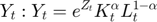
Response variable Consumption ( $C$ ), Labor ( $L$ ), Marginal utility with respect to consumption ( $U_C$ ), Instantaneous utility ( $U$ ), Production ( $Y$ ), Utility ( $V$ ).

State variable Capital stock ( $K$ ), Log of productivity ( $Z$ ), Log of productivity volatility ( $\sigma$ ).

Shock Innovation to productivity ( $\epsilon$ ), Innovation to productivity volatility ( $\omega$ ).

Parameters Capital depreciation rate ( $\delta$ ), Discount factor ( $\beta$ ), Index of deviation from CRRA utility ( $\nu$ ), Risk-aversion parameter ( $\tau$ ), Capital share ( $\alpha$ ), Share of consumption in utility ( $\theta$ ), Persistence of log-productivity ( $\rho_Z$ ), Persistence of SV ( $\rho_{\sigma}$ ), Unconditional mean of SV ( $\bar{\sigma}$ ), Standard deviation of SV ( $\eta$ ).

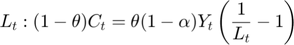
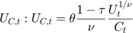
Equilibrium equation

$C_{t}: U_{C,t}=\beta\left(\mathrm{E}_{t}\tilde{V}_{t+1}\right)^{\left(\frac{1}{\theta}-1\right)}\mathrm{E}_{t}\left[\tilde{V}_{t+1}^{\frac{\theta-1}{\theta}}U_{C,t+1}\left(1-\delta+ \alpha e^{Z_{t+1}}K_{t+1}^{\alpha-1}L_{t+1}^{\alpha-1}\right)\right].$

$L_t: (1-\theta) C_t = \theta (1-\alpha) Y_t \left(\frac{1}{L_t}-1\right)$

$U_{C,t}: U_{C,t} = \theta \frac{1-\tau}{\nu} \frac{U_t^{1/\nu}}{C_t}$

$U_t: U_t = \left[C_t^{\theta}(1-L_t)^{1-\theta}\right]^{1-\tau}$

$Y_t: Y_t = e^{Z_{t}}K_{t}^{\alpha}L_t^{1-\alpha}$

$V_t: \tilde{V}_t^{\frac{1}{\nu}} = (1-\beta) U_t^{\frac{1}{\nu}} + \beta \mathrm{E}_t \tilde{V}_t^{\frac{1}{\nu}}$

$\tilde{V}_t: \tilde{V}_t=V_t^{1-\tau}$

Transition equations

$K_{t}: K_{t}=+\left(1-\delta\right)K_{t-1}-C_{t-1},$

$Z_{t}: Z_{t}=\rho_Z Z_{t-1}+e^{\sigma_t}\epsilon_{t}.$

$\sigma_t: \sigma_t = (1-\rho_{\sigma})\bar{\sigma}+\rho_{\sigma}\sigma_{t-1}+\eta\omega_t$

Writing the model

The model is defined in a Yaml file: gro3.yaml.

Create the model object

model = recsmodel('gro3.yaml',struct('Mu',[0 0],'Sigma',eye(2),'order',5));

Deterministic steady state (different from first guess, max(|delta|)=0.74174)
 State variables:
      K            Z          Sigma 
    ______    ___________    _______

    9.3926    -2.3527e-18    -4.9618

 Response variables:
       C          L         Uc          U          Y          V         Vt   
    _______    _______    _______    _______    _______    _______    _______

    0.71389    0.32835    0.20716    0.82851    0.89799    0.68644    0.82851

 Expectations variables:
      EC         EVt  
    _______    _______

    0.20904    0.82851

Define approximation space using Chebyshev polynomials

smin       = [0.85*model.sss(1) -0.11 log(0.007)*1.15];
smax       = [1.20*model.sss(1)  0.11 log(0.007)*0.85];

[interp,s] = recsinterpinit(4,smin,smax,'cheb');

Find a first guess through first-order approximation around the steady state

[interp,x] = recsFirstGuess(interp,model,s);

Define options

options = struct('reemethod','1-step',...
                 'accuracy' ,1,...
                 'stat'     ,1);

Solve for rational expectations

[interp,x,z] = recsSolveREE(interp,model,s,x,options);

Use simple continuation method to solve for higher values of risk aversion

The procedure to solve for different parameters values has to be packed in a function. This is done in gro3problem.m.

type('gro3problem.m')

function [X,f,exitflag] = gro3problem(X,z)
% GRO3PROBLEM Solves the model GRO3 for different values of risk aversion and IES

[model,interp,s,x,options] = X{:};

tau = z(1);
Psi = z(2);
nu  = (1-tau)/(1-1/Psi);
model.params(1)         = tau;
model.params(end-1:end) = [nu Psi];

[interp,x,~,f,exitflag] = recsSolveREE(interp,model,s,x,options);

X = {model interp s x options};

This function requires as input the cell array X:

X = {model interp s x options};

The function SCP starts from the known solution with a low risk aversion to find in 2 steps the solution with an higher risk aversion:

X = SCP(X,[5 0.5],[0.5 1/0.5],@gro3problem,2);
[model,interp,s,x,options] = X{:};

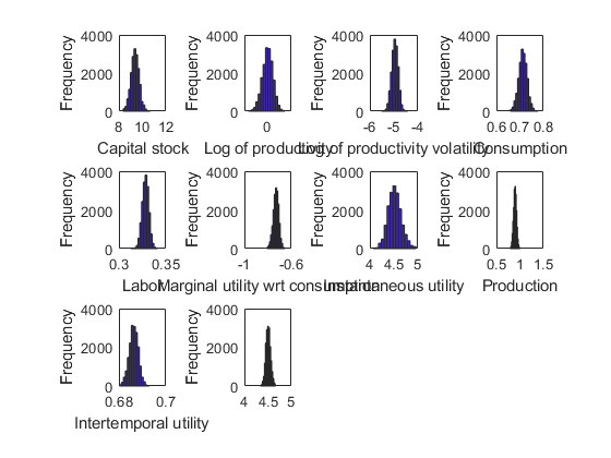
Simulate the model

recsSimul(model,interp,model.sss(ones(100,1),:),200,[],options);
subplot(3,4,1)
xlabel('Capital stock')
ylabel('Frequency')
subplot(3,4,2)
xlabel('Log of productivity')
ylabel('Frequency')
subplot(3,4,3)
xlabel('Log of productivity volatility')
ylabel('Frequency')
subplot(3,4,4)
xlabel('Consumption')
ylabel('Frequency')
subplot(3,4,5)
xlabel('Labor')
ylabel('Frequency')
subplot(3,4,6)
xlabel('Marginal utility wrt consumption')
ylabel('Frequency')
subplot(3,4,7)
xlabel('Instantaneous utility')
ylabel('Frequency')
subplot(3,4,8)
xlabel('Production')
ylabel('Frequency')
subplot(3,4,9)
xlabel('Intertemporal utility')
ylabel('Frequency')
subplot(3,4,10)
xlabel('')
ylabel('Frequency')

Statistics from simulated variables (excluding the first 20 observations):
 Moments
                Mean        StdDev      Skewness     Kurtosis       Min         Max       pLB    pUB
             __________    _________    _________    ________    _________    ________    ___    ___

    K            9.3726       0.3448     0.049759    3.1699         8.3612      10.667    NaN    NaN
    Z        -0.0010056     0.022278     -0.12717    3.0141      -0.082602    0.072685    NaN    NaN
    Sigma       -4.9589      0.13472    -0.079306    2.9814        -5.5057     -4.4161    NaN    NaN
    C           0.71284     0.017722    -0.020588    3.0338        0.65859     0.77676      0      0
    L           0.32833    0.0035491    -0.086214    3.1091         0.3127     0.34121      0      0
    Uc         -0.73063      0.02345     -0.19052    3.0803       -0.80705    -0.65302      0      0
    U            4.5172      0.13699      0.17868    3.1564         4.0595       4.959      0      0
    Y           0.89685     0.032524     -0.01658     2.985        0.79054      1.0092      0      0
    V           0.68632    0.0019234    -0.084775    3.0172        0.68021     0.69296      0      0
    Vt           4.5073     0.050563      0.12709    3.0239         4.3367      4.6713      0      0

 Correlation
                K           Z          Sigma         C            L           Uc           U           Y           V           Vt    
             ________    ________    _________    ________    _________    ________    _________    ________    ________    _________

    K               1     0.62478     0.046136     0.93156      0.20961     0.95867     -0.99857     0.73116     0.90316     -0.90282
    Z         0.62478           1     0.026014     0.86584      0.89427     0.81844     -0.61567     0.98918     0.89935     -0.89944
    Sigma    0.046136    0.026014            1    0.041852    0.0065812    0.043077    -0.046003    0.032588    0.040492    -0.040309
    C         0.93156     0.86584     0.041852           1      0.55058     0.99528     -0.92653     0.92909     0.99737     -0.99717
    L         0.20961     0.89427    0.0065812     0.55058            1     0.47492     -0.19805     0.82003     0.60862     -0.60875
    Uc        0.95867     0.81844     0.043077     0.99528      0.47492           1     -0.95661     0.89201     0.98696     -0.98715
    U        -0.99857    -0.61567    -0.046003    -0.92653     -0.19805    -0.95661            1    -0.72241    -0.89796      0.89806
    Y         0.73116     0.98918     0.032588     0.92909      0.82003     0.89201     -0.72241           1     0.95285     -0.95267
    V         0.90316     0.89935     0.040492     0.99737      0.60862     0.98696     -0.89796     0.95285           1     -0.99995
    Vt       -0.90282    -0.89944    -0.040309    -0.99717     -0.60875    -0.98715      0.89806    -0.95267    -0.99995            1

 Autocorrelation
               T1         T2         T3         T4         T5   
             _______    _______    _______    _______    _______

    K        0.99495    0.98532    0.97156    0.95413    0.93348
    Z        0.92544    0.85546    0.78812    0.72396    0.66418
    Sigma    0.87737    0.77009    0.67678    0.59627    0.52422
    C        0.97313    0.94488    0.91479    0.88323    0.85085
    L        0.90432    0.81569    0.73158    0.65263    0.58046
    Uc       0.98183    0.96106    0.93766    0.91191     0.8844
    U        0.99481    0.98507    0.97118    0.95365    0.93291
    Y        0.93633    0.87596    0.81718    0.76052    0.70699
    V        0.96592     0.9314    0.89576    0.85936    0.82292
    Vt       0.96594    0.93144    0.89583    0.85946    0.82304

Accuracy of the solution
 Equilibrium equation error (in log10 units)
    Max       Mean
   -5.3396   -5.6612
   -5.4924   -5.9614
   -4.7854   -5.0195
   -3.5812   -3.7903
   -5.0962   -5.4858
   -6.8940   -7.1197
   -5.3354   -5.5530

References

Caldara D.; Fernandez-Villaverdes, J.; Rubio-Ramirez, J. F. & Yao, W. (2012). Computing DSGE models with recursive preferences and stochastic volatility. Review of Economic Dynamics 15(2), 188-206.

RECS