STO2 Competitive storage with floor-price backed by public storage

This model is close to one of the models presented in Wright and Williams (1988).

Model's structure

Response variables Speculative storage ($S^{\mathrm{S}}$), Public storage ($S^{\mathrm{G}}$), Planned production ($H$) and Price ($P$).

State variable Availability ($A$).

Shock Productivity shocks ($\epsilon$).

Parameters Unit physical storage cost ($k$), Depreciation share ($\delta$), Interest rate ($r$), Scale parameter for the production cost function ($h$), Inverse of supply elasticity ($\mu$), Demand price elasticity ($\alpha$), Floor price ($P^{\mathrm{F}}$) and Capacity constraint on public stock ($\bar{S}^{\mathrm{G}}$).

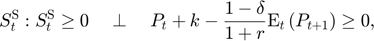
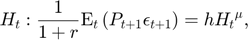
Equilibrium equations

$S^{\mathrm{S}}_{t}: S^{\mathrm{S}}_{t}\ge 0 \quad \perp \quad P_{t}+k-\frac{1-\delta}{1+r}\mathrm{E}_{t}\left(P_{t+1}\right)\ge 0,$

$H_{t}: \frac{1}{1+r}\mathrm{E}_{t}\left(P_{t+1}\epsilon_{t+1}\right)=h {H_{t}}^{\mu},$

$P_{t}: A_{t}={P_{t}}^{\alpha}+S^{\mathrm{S}}_{t}+S^{\mathrm{G}}_{t},$

$S^{\mathrm{G}}_{t}: 0\le S^{\mathrm{G}}_{t}\le \bar{S}^{\mathrm{G}} \quad \perp \quad P_t - P^{\mathrm{F}}.$

Transition equation

$A_{t}: A_{t}=\left(1-\delta\right)\left(S^{\mathrm{S}}_{t-1}+S^{\mathrm{G}}_{t-1}\right)+H_{t-1}\epsilon_{t}.$

Writing the model

The model is defined in a Yaml file: sto2.yaml.

Create the model object

Mu                = 1;
sigma             = 0.05;
model = recsmodel('sto2.yaml',struct('Mu',Mu,'Sigma',sigma^2,'order',7));

Deterministic steady state (different from first guess, max(|delta|)=0.392101)
 State variables:
      A   
    ______

    1.3921

 Response variables:
        S           H       P        Sg   
    __________    _____    ____    _______

    6.0863e-15    1.004    1.02    0.39605

 Expectations variables:
     EP     EPe 
    ____    ____

    1.02    1.02

Define approximation space

[interp,s] = recsinterpinit(50,0.7,2);

Find a first guess through the perfect foresight solution

interp = recsFirstGuess(interp,model,s,model.sss,model.xss,struct('T',5));

Solve for rational expectations

[interp,x] = recsSolveREE(interp,model,s);

Successive approximation
  Major	 Minor	Lipschitz	 Residual
      0	     0	         	 3.02E-02 (Input point)
      1	     1	  1.0269	 1.39E-02
      2	     1	  0.9062	 8.27E-03
      3	     1	  0.9942	 1.07E-03
      4	     1	  1.0897	 5.32E-04
      5	     1	  0.7831	 1.17E-04
      6	     1	  0.8366	 1.91E-05
      7	     1	  0.8449	 2.97E-06
      8	     1	  0.8459	 4.57E-07
      9	     1	  0.8460	 7.04E-08
     10	     1	  1.0000	 0.00E+00
Solution found - Residual lower than absolute tolerance

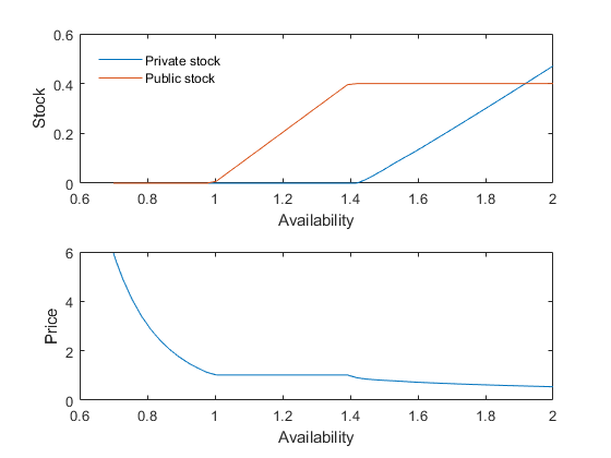
Plot storage and price rules

subplot(2,1,1)
plot(s,x(:,[1 4]))
leg = legend('Private stock','Public stock');
set(leg,'Location','NorthWest')
set(leg,'Box','off')
xlabel('Availability')
ylabel('Stock')
subplot(2,1,2)
plot(s,x(:,3))
xlabel('Availability')
ylabel('Price')

References

Wright, B. D. and Williams, J. C. (1988). The incidence of market-stabilising price support schemes. The Economic Journal, 98(393), 1183-1198.