STO5 Two-country storage-trade model

Model close to Miranda and Glauber (1995). Countries $a$ and $b$ are indicated by the subscript $i \in \left\{a,b\right\}$ . When variables corresponding to both countries appear in the same equation, the foreign country is indicated by the subscript $j$ .

Model's structure
Writing the model
Create the model object
Define approximation space
Find a first guess through the perfect foresight solution
Solve for rational expectations
Simulate the model
References

Model's structure

Response variables Storage ( $S_{i}$ ), Planned production ( $H_{i}$ ), Price ( $P_{i}$ ) and Export ( $X_{i}$ ).

State variable Availability ( $A_{i}$ ).

Shock Productivity shocks ( $\epsilon_{i}$ ).

Parameters Unit physical storage cost ( $k$ ), Depreciation share ( $\delta$ ), Interest rate ( $r$ ), Scale parameter for the production cost function ( $h$ ), Inverse of supply elasticity ( $\mu$ ), Demand price elasticity ( $\alpha$ ), Scale parameter for demand function ( $\gamma_i$ ), Trade cost ( $\theta$ ) and Tariff ( $\tau_{i}$ ).

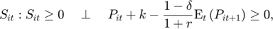
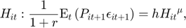
Equilibrium equations

For $i \in \left\{a,b\right\}$ and $j \ne i$ :

$S_{it}: S_{it}\ge 0 \quad \perp \quad P_{it}+k-\frac{1-\delta}{1+r}\mathrm{E}_{t}\left(P_{it+1}\right)\ge 0,$

$H_{it}: \frac{1}{1+r}\mathrm{E}_{t}\left(P_{it+1}\epsilon_{it+1}\right)=h {H_{it}}^{\mu},$

$P_{it}: A_{it}+X_{jt}=\gamma_i{P_{it}}^{\alpha}+S_{it}+X_{it},$

$X_{it}: X_{it}\ge 0 \quad \perp \quad P_{it}+\theta+\tau_{j}\ge P_{jt}.$

Transition equation

For $i \in \left\{a,b\right\}$ :

$A_{it}: A_{it}=\left(1-\delta\right)S_{it-1}+H_{it-1}\epsilon_{it}.$

Writing the model

The model is defined in a Yaml file: sto5.yaml.

Create the model object

Mu                = [1 1];
sigma             = [0.05 0;
                     0    0.05];
model = recsmodel('sto5.yaml',struct('Mu',Mu,'Sigma',sigma^2,'order',7));

Deterministic steady state (different from first guess, max(|delta|)=0.31777)
 State variables:
      Aa        Ab  
    ______    ______

    1.0402    1.0567

 Response variables:
    Sa        Sb          Ha        Hb        Pa        Pb         Xa       Xb
    __    __________    ______    ______    ______    ______    ________    __

    0     8.4168e-19    1.0402    1.0567    1.2178    1.3178    0.078829    0 

 Expectations variables:
     EPa       EPb       EPea      EPeb 
    ______    ______    ______    ______

    1.2178    1.3178    1.2178    1.3178

Define approximation space

[interp,s] = recsinterpinit(15,0.73*model.sss,2*model.sss);

Find a first guess through the perfect foresight solution

interp = recsFirstGuess(interp,model,s,model.sss,model.xss,struct('T',5));

Solve for rational expectations

[interp,x] = recsSolveREE(interp,model,s);

Successive approximation
  Major	 Minor	Lipschitz	 Residual
      0	     0	         	 7.73E-01 (Input point)
      1	     1	  0.8943	 2.14E-01
      2	     1	  0.9616	 9.75E-02
      3	     1	  0.7867	 7.31E-02
      4	     1	  0.6319	 4.34E-02
      5	     1	  0.6484	 1.69E-02
      6	     1	  0.7361	 4.49E-03
      7	     1	  0.7768	 1.00E-03
      8	     1	  0.7905	 2.10E-04
      9	     1	  0.7945	 4.32E-05
     10	     1	  0.7958	 8.82E-06
     11	     1	  0.7962	 1.80E-06
     12	     1	  0.8031	 3.74E-07
     13	     1	  0.9038	 8.46E-08
     14	     1	  1.0000	 0.00E+00
Solution found - Residual lower than absolute tolerance

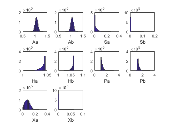
Simulate the model

[~,~,~,stat] = recsSimul(model,interp,model.sss(ones(1E4,1),:),100);

Statistics from simulated variables (excluding the first 20 observations):
 Moments
             Mean         StdDev      Skewness     Kurtosis      Min        Max         pLB      pUB
          __________    __________    _________    ________    _______    ________    _______    ___

    Aa        1.0615      0.056021     0.079139    3.0594      0.82001       1.342        NaN    NaN
    Ab        1.0588      0.053172    0.0023208         3      0.78352      1.3038        NaN    NaN
    Sa      0.021354       0.02686       1.7747    6.5435            0     0.26334     20.218      0
    Sb     0.0014208     0.0049854       6.2295    57.578            0     0.11381     70.087      0
    Ha        1.0406      0.005748      -1.4948    5.0673       1.0027      1.0463          0      0
    Hb        1.0574     0.0054542      -1.5047    5.0917       1.0214      1.0628          0      0
    Pa        1.2222       0.17537       1.5246    6.0402      0.90647      3.1226          0      0
    Pb        1.3242       0.17191       1.5469    6.4956      0.99882      3.2159          0      0
    Xa      0.077861      0.038788      0.33209    2.6835            0     0.26816    0.15363      0
    Xb    0.00016171    0.00086318       23.532    798.22            0    0.061958     44.815      0

 Correlation
             Aa           Ab           Sa           Sb           Ha          Hb          Pa          Pb          Xa          Xb    
          _________    _________    _________    _________    ________    ________    ________    ________    ________    _________

    Aa            1    -0.032507      0.68347    -0.084515    -0.64564    -0.64578    -0.66163    -0.66965     0.52251     -0.20812
    Ab    -0.032507            1      0.53128      0.52702      -0.605    -0.60358    -0.63603    -0.63559    -0.84956       0.1135
    Sa      0.68347      0.53128            1       0.1961    -0.98168    -0.98219    -0.65901    -0.67349      -0.182    -0.060681
    Sb    -0.084515      0.52702       0.1961            1    -0.36548    -0.36373    -0.21845    -0.22125     -0.4213      0.07748
    Ha     -0.64564       -0.605     -0.98168     -0.36548           1     0.99999     0.68427      0.6972     0.24316     0.055652
    Hb     -0.64578     -0.60358     -0.98219     -0.36373     0.99999           1     0.68284     0.69585     0.24239      0.05576
    Pa     -0.66163     -0.63603     -0.65901     -0.21845     0.68427     0.68284           1     0.99549     0.15623      0.10826
    Pb     -0.66965     -0.63559     -0.67349     -0.22125      0.6972     0.69585     0.99549           1     0.15001     0.047489
    Xa      0.52251     -0.84956       -0.182      -0.4213     0.24316     0.24239     0.15623     0.15001           1     -0.16019
    Xb     -0.20812       0.1135    -0.060681      0.07748    0.055652     0.05576     0.10826    0.047489    -0.16019            1

 Autocorrelation
              T1           T2           T3           T4           T5    
          __________    _________    _________    _________    _________

    Aa       0.22939      0.02947    -0.010715     -0.01749    -0.020583
    Ab     -0.028468    -0.024722     -0.01517    -0.012473    -0.012601
    Sa        0.1978     0.022797    -0.011241    -0.017322    -0.018987
    Sb     0.0060039    -0.016106    -0.014682    -0.013809     -0.01206
    Ha       0.18214     0.019869    -0.011336    -0.017478    -0.018262
    Hb       0.18243      0.01992    -0.011329    -0.017489    -0.018273
    Pa       0.10913    0.0078086    -0.013164    -0.016746    -0.016546
    Pb       0.11533    0.0090659    -0.013051    -0.016779    -0.016571
    Xa     -0.030315    -0.026361    -0.015005    -0.011474    -0.013226
    Xb    -0.0053893    -0.011814    -0.013243     -0.01292    -0.013993

References

Miranda, M. J. and Glauber, J. W. (1995). Solving stochastic models of competitive storage and trade by Chebychev collocation methods. Agricultural and Resource Economics Review, 24(1), 70-77.

RECS