STO6 Quarterly storage model with annual inelastic supply
This model represents the market of a storable commodity that is produced once a year and stored for a year-long consumption. Supply is stochastic and inelastic. Except for its distribution, no information about the coming harvest is known.
Contents
Model's structure
Writing the model
The model is defined in a Yaml file: sto6.yaml.
Create the model object
model = recsmodel('sto6.yaml',struct('Mu',0,'Sigma',0.05^2,'order',5));
Deterministic steady state (different from first guess, max(|delta|)=0.0961408)
 State variables:
    A1
    __

    4

 Response variables:
      S1        S2        S3           S4          P1         P2        P3        P4        A2        A3        A4
    ______    ______    _______    __________    _______    ______    ______    ______    ______    ______    _______

    2.9964    1.9854    0.98671    1.9961e-18    0.98214    1.0197    1.0577    1.0961    2.9815    1.9756    0.98181

 Expectations variables:
      EP
    _______

    0.98214
Define approximation space
interp = recsinterpinit(50,model.sss*0.7,model.sss*1.5);
Find a first guess through the perfect foresight solution
interp = recsFirstGuess(interp,model);
Solve for rational expectations
[interp,Xcat] = recsSolveREE(interp,model);
Successive approximation
  Major	 Minor	Lipschitz	 Residual
      0	     0	         	 7.61E-02 (Input point)
      1	     1	  0.7086	 4.93E-02
      2	     1	  0.5706	 3.31E-02
      3	     1	  0.5590	 1.55E-02
      4	     1	  0.6546	 5.38E-03
      5	     1	  0.6941	 1.65E-03
      6	     1	  0.7079	 4.81E-04
      7	     1	  0.7122	 1.38E-04
      8	     1	  0.7151	 3.94E-05
      9	     1	  0.7159	 1.12E-05
     10	     1	  0.7163	 3.18E-06
     11	     1	  0.7161	 9.03E-07
     12	     1	  0.7157	 2.57E-07
     13	     1	  1.0000	 0.00E+00
Solution found - Residual lower than absolute tolerance
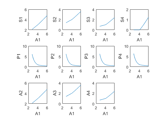
Plot the decision rules
recsDecisionRules(model,interp,[],[],[],struct('simulmethod','solve'));
for i=1:model.dim{2}
  subplot(3,4,i)
  xlabel(model.symbols.states{1});
  ylabel(model.symbols.controls{i});
end
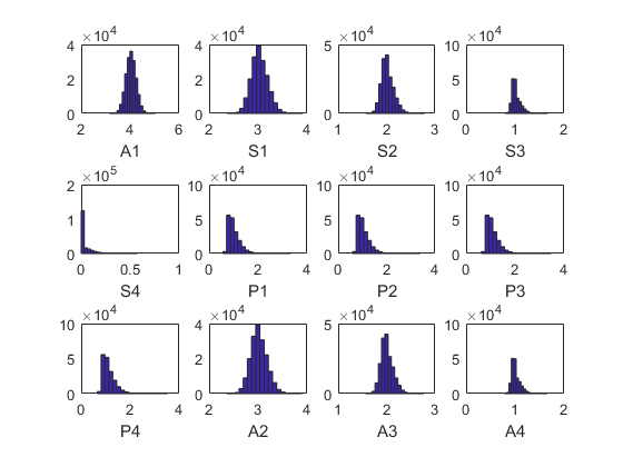
Simulate the model
[ssim,~,~,stat] = recsSimul(model,interp,model.sss(ones(1000,1),:),200,[],...
                            struct('accuracy',1));
subplot(3,4,1)
xlabel(model.symbols.states{1});
for i=1:model.dim{2}
  subplot(3,4,i+1)
  xlabel(model.symbols.controls{i});
end
Statistics from simulated variables (excluding the first 20 observations):
 Moments
            Mean       StdDev     Skewness    Kurtosis      Min        Max       pLB      pUB
          ________    ________    ________    ________    _______    _______    ______    ___

    A1      4.0339     0.20819    0.045874    3.0194       3.1503     5.0401       NaN    NaN
    S1      3.0303      0.1669     0.25675    3.1639       2.3639     3.9152         0      0
    S2      2.0193     0.12679     0.60361    3.5534       1.5689     2.7836         0      0
    S3      1.0207    0.089673      1.2152    4.7192      0.78099     1.6694         0      0
    S4    0.034219    0.058308      2.1537    8.0546            0    0.57222    27.647      0
    P1      1.0112     0.23947      1.4769    6.0874      0.55524     3.3258         0      0
    P2      1.0491     0.24245      1.4769    6.0874      0.58746     3.3925         0      0
    P3      1.0875     0.24546      1.4769    6.0874      0.62008       3.46         0      0
    P4      1.1263     0.24852      1.4769    6.0874      0.65311     3.5283         0      0
    A2      3.0153     0.16607     0.25675    3.1639       2.3522     3.8958         0      0
    A3      2.0093     0.12616     0.60361    3.5534       1.5612     2.7697         0      0
    A4      1.0156    0.089228      1.2152    4.7192      0.77712     1.6612         0      0

 Correlation
             A1          S1          S2          S3          S4          P1          P2          P3          P4          A2          A3          A4
          ________    ________    ________    ________    ________    ________    ________    ________    ________    ________    ________    ________

    A1           1     0.99865      0.9908     0.95879     0.81734    -0.93754    -0.93754    -0.93754    -0.93754     0.99865      0.9908     0.95879
    S1     0.99865           1     0.99649     0.97225     0.84617    -0.91938    -0.91938    -0.91938    -0.91938           1     0.99649     0.97225
    S2      0.9908     0.99649           1     0.98842     0.88781    -0.88482    -0.88482    -0.88482    -0.88482     0.99649           1     0.98842
    S3     0.95879     0.97225     0.98842           1     0.94735    -0.80621    -0.80621    -0.80621    -0.80621     0.97225     0.98842           1
    S4     0.81734     0.84617     0.88781     0.94735           1    -0.57807    -0.57807    -0.57807    -0.57807     0.84617     0.88781     0.94735
    P1    -0.93754    -0.91938    -0.88482    -0.80621    -0.57807           1           1           1           1    -0.91938    -0.88482    -0.80621
    P2    -0.93754    -0.91938    -0.88482    -0.80621    -0.57807           1           1           1           1    -0.91938    -0.88482    -0.80621
    P3    -0.93754    -0.91938    -0.88482    -0.80621    -0.57807           1           1           1           1    -0.91938    -0.88482    -0.80621
    P4    -0.93754    -0.91938    -0.88482    -0.80621    -0.57807           1           1           1           1    -0.91938    -0.88482    -0.80621
    A2     0.99865           1     0.99649     0.97225     0.84617    -0.91938    -0.91938    -0.91938    -0.91938           1     0.99649     0.97225
    A3      0.9908     0.99649           1     0.98842     0.88781    -0.88482    -0.88482    -0.88482    -0.88482     0.99649           1     0.98842
    A4     0.95879     0.97225     0.98842           1     0.94735    -0.80621    -0.80621    -0.80621    -0.80621     0.97225     0.98842           1

 Autocorrelation
            T1          T2          T3            T4            T5
          _______    ________    _________    __________    __________

    A1    0.21648    0.047568    0.0089635     -0.006843     -0.008623
    S1    0.22687    0.050773    0.0094296    -0.0070417    -0.0089489
    S2    0.24164    0.055368     0.010032    -0.0073559    -0.0094548
    S3     0.2611    0.061608     0.010651    -0.0078625     -0.010267
    S4    0.26473    0.064139    0.0099399    -0.0083125     -0.011228
    P1    0.13189    0.022645    0.0049882    -0.0058688    -0.0070509
    P2    0.13189    0.022645    0.0049882    -0.0058688    -0.0070509
    P3    0.13189    0.022645    0.0049882    -0.0058688    -0.0070509
    P4    0.13189    0.022645    0.0049882    -0.0058688    -0.0070509
    A2    0.22687    0.050773    0.0094296    -0.0070417    -0.0089489
    A3    0.24164    0.055368     0.010032    -0.0073559    -0.0094548
    A4     0.2611    0.061608     0.010651    -0.0078625     -0.010267

Accuracy of the solution
 Equilibrium equation error (in log10 units)
    Max       Mean
   -8.0300   -8.6895
   -8.3915   -9.3227
   -8.5612   -9.2494
   -2.1736   -3.1645
   -4.6787   -5.3781
   -4.7071   -5.4060
   -4.7345   -5.4329
   -3.3738   -4.4109
  -14.6536  -15.4064
  -14.8754  -15.6120
  -15.1764  -15.8576