CS1 Consumption/saving model with borrowing constraint

This is an implementation of the model in Deaton (1991).

Model's structure

Response variable Consumption ($C$).

State variable Cash on hand ($X$).

Shock Labor income ($Y$).

Parameters Interest rate ($r$), Rate of time preference ($\delta$), and Elasticity of intertemporal substitution ($\rho$).

Equilibrium equation

$C_{t}: C_{t}\le X_{t} \quad \perp \quad \frac{1+r}{1+\delta}\mathrm{E}_{t}\left(C_{t+1}^{-\rho}\right)-C_{t}^{-\rho}\le 0.$

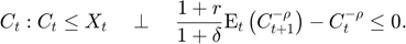
Transition equation

$X_{t}: X_{t}=\left(1+r\right)\left(X_{t-1}-C_{t-1}\right)+Y_{t}.$

Writing the model

The model is defined in a Yaml file: cs1.yaml.

Create the model object

Mean and standard deviation of the shocks

Mu                = 100;
sigma             = 10;

You generate the MATLAB model file and pack the model object with the following command

model = recsmodel('cs1.yaml',...
                  struct('Mu',Mu,'Sigma',sigma^2,'order',5));

Deterministic steady state (equal to first guess)
 State variables:
     X 
    ___

    100

 Response variables:
     C 
    ___

    100

 Expectations variables:
      E   
    ______

    0.0001

This command creates a MATLAB file, cs1model.m, containing the definition the model and all its Jacobians from the human readable file cs1.yaml.

Define approximation space

[interp,s] = recsinterpinit(20,model.sss/2,model.sss*2);

First-guess: Consumption equal to cash on hand

x         = s;

To force the solver to compute the approximation of the expectations function, it is necessary to add at least an empty value for interp.ch

interp.ch = [];

Solve for rational expectations

[interp,x] = recsSolveREE(interp,model,s,x);

Successive approximation
  Major	 Minor	Lipschitz	 Residual
      0	     0	         	 1.08E+02 (Input point)
      1	     1	  0.6916	 3.35E+01
      2	     1	  0.5517	 1.50E+01
      3	     1	  0.4800	 7.82E+00
      4	     1	  0.4413	 4.37E+00
      5	     1	  0.4210	 2.53E+00
      6	     1	  0.4128	 1.49E+00
      7	     1	  0.4128	 8.74E-01
      8	     1	  0.4145	 5.12E-01
      9	     1	  0.4179	 2.98E-01
     10	     1	  0.4232	 1.72E-01
     11	     1	  1.0000	 0.00E+00
Solution found - Residual lower than absolute tolerance

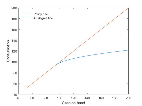
Plot the decision rule

figure
plot(s,[x s])
legend('Policy rule','45 degree line')
legend('Location','NorthWest')
legend('boxoff')
xlabel('Cash on hand')
ylabel('Consumption')

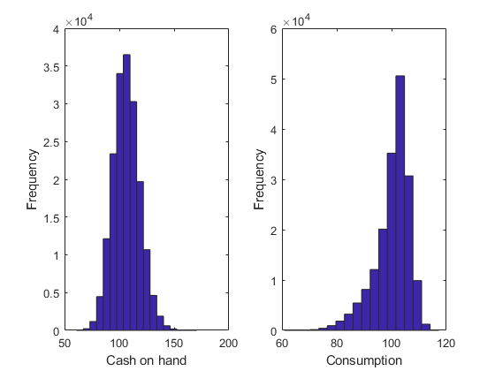
Simulate the model

[~,~,~,stat] = recsSimul(model,interp,model.sss(ones(1000,1),:),200);
subplot(1,2,1)
xlabel('Cash on hand')
ylabel('Frequency')
subplot(1,2,2)
xlabel('Consumption')
ylabel('Frequency')

Statistics from simulated variables (excluding the first 20 observations):
 Moments
          Mean     StdDev    Skewness    Kurtosis     Min       Max      pLB     pUB  
         ______    ______    ________    ________    ______    ______    ___    ______

    X    106.46    11.993    0.21404     3.1685      60.906    170.81    NaN       NaN
    C     100.3    6.3358    -1.2064     4.8722      60.904    117.21      0    12.001

 Correlation
            X          C   
         _______    _______

    X          1    0.94694
    C    0.94694          1

 Autocorrelation
           T1         T2         T3          T4          T5   
         _______    _______    _______    ________    ________

    X    0.50523    0.26951    0.14663    0.073857    0.035042
    C    0.38738    0.19105    0.10297    0.049875    0.022239

References

Deaton, A. (1991). Saving and liquidity constraints. Econometrica, 59(5), 1221-1248.