GRO1 Stochastic growth model

Model's structure
Writing the model
Create the model object
Define approximation space using Chebyshev polynomials
Find a first guess through first-order approximation around the steady state
Define options
Solve for rational expectations
Simulate the model

Model's structure

Response variable Consumption ( $C$ ).

State variable Capital stock ( $K$ ), Log of productivity ( $Z$ ).

Shock Innovation to productivity ( $\epsilon$ ).

Parameters Capital depreciation rate ( $\delta$ ), Discount factor ( $\beta$ ), Elasticity of intertemporal substitution ( $\tau$ ), Capital share ( $\alpha$ ), Scale parameter ( $a$ ).

Equilibrium equation

$C_{t}: C_{t}^{-\tau}=\beta\mathrm{E}_{t}\left[C_{t+1}^{-\tau}\left(1-\delta+a \alpha e^{Z_{t+1}}K_{t+1}^{\alpha-1}\right)\right].$

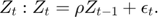
Transition equations

$K_{t}: K_{t}=a e^{Z_{t-1}}K_{t-1}^{\alpha}+\left(1-\delta\right)K_{t-1}-C_{t-1},$

$Z_{t}: Z_{t}=\rho Z_{t-1}+\epsilon_{t}.$

Writing the model

The model is defined in a Yaml file: gro1.yaml.

Create the model object

Mean and standard deviation of the shocks

Mu                = 0;
sigma             = 0.007;

You generate the MATLAB model file and pack the model object with the following command

model = recsmodel('gro1.yaml',...
                  struct('Mu',Mu,'Sigma',sigma^2,'order',5));

Deterministic steady state (different from first guess, max(|delta|)=1.75094e-08)
 State variables:
    K        Z    
    _    _________

    1    3.216e-22

 Response variables:
       C   
    _______

    0.19928

 Expectations variables:
      E   
    ______

    26.505

This command creates a MATLAB file, gro1model.m, containing the definition the model and all its Jacobians from the human readable file gro1.yaml.

Define approximation space using Chebyshev polynomials

Degree of approximation

order         = [10 10];

Limits of the state space

smin          = [0.85*model.sss(1) min(model.shocks.e)*4];
smax          = [1.15*model.sss(1) max(model.shocks.e)*4];

[interp,s] = recsinterpinit(order,smin,smax,'cheb');

Find a first guess through first-order approximation around the steady state

[interp,x] = recsFirstGuess(interp,model,s,model.sss,model.xss);

Define options

With high order Chebyshev polynomials, extrapolation outside the state space should not be allowed to prevent explosive values.

options = struct('reesolver','krylov',...
                 'extrapolate',0    ,...
                 'accuracy'   ,1);

Solve for rational expectations

interp = recsSolveREE(interp,model,s,x,options);

Newton-Krylov solver
  Major  Residual  Minor 1  Relative res.  Minor 2
      0  1.32E-04        0       1.00E+00        0 (Input point)
      1  2.70E-05        1       2.04E-01        0
      2  1.88E-05        1       6.97E-01        0
      3  2.80E-06        2       1.49E-01        0
      4  4.97E-08        3       1.78E-02        0
      5  1.12E-09        4       2.26E-02        0

Simulate the model

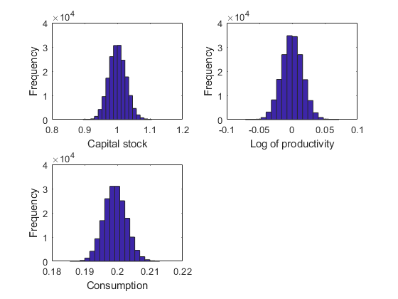
[~,~,~,stat] = recsSimul(model,interp,model.sss(ones(1000,1),:),200,[],options);
subplot(2,2,1)
xlabel('Capital stock')
ylabel('Frequency')
subplot(2,2,2)
xlabel('Log of productivity')
ylabel('Frequency')
subplot(2,2,3)
xlabel('Consumption')
ylabel('Frequency')

Statistics from simulated variables (excluding the first 20 observations):
 Moments
            Mean         StdDev      Skewness     Kurtosis       Min         Max       pLB    pUB
         ___________    _________    _________    ________    _________    ________    ___    ___

    K         1.0007     0.026494      0.11057    3.0062        0.89474      1.1053    NaN    NaN
    Z    -3.3217e-05     0.015946    0.0022828    2.9987      -0.071637    0.071787    NaN    NaN
    C        0.19934    0.0034279     0.078804     2.989        0.18546     0.21301      0      0

 Correlation
            K          Z          C   
         _______    _______    _______

    K          1    0.52294    0.94816
    Z    0.52294          1    0.76667
    C    0.94816    0.76667          1

 Autocorrelation
           T1         T2         T3         T4         T5   
         _______    _______    _______    _______    _______

    K    0.99396    0.98004    0.95955    0.93366    0.90339
    Z     0.8772     0.7681    0.67239    0.58658    0.51118
    C     0.9733    0.94265    0.90909    0.87289    0.83506

Accuracy of the solution
 Equilibrium equation error (in log10 units)
    Max       Mean
   -2.9649   -4.9531

RECS