GRO2 Stochastic growth model with irreversible investment

This is an implementation of the model in Christiano and Fisher (2000).

Model's structure

Response variable Consumption ($C$), Investment ($I$), Lagrange multiplier ($\mu$).

State variable Capital stock ($K$), Log of productivity ($Z$).

Shock Innovation to productivity ($\epsilon$).

Parameters Capital depreciation rate ($\delta$), Discount factor ($\beta$), Elasticity of intertemporal substitution ($\tau$), Capital share ($\alpha$), Scale parameter ($a$).

Equilibrium equations

$C_{t}: C_{t}+I_{t}=a e^{Z_{t}}K_{t}^{\alpha},$

$I_{t}:I_{t}\ge 0 \quad \perp \quad C_{t}^{-\tau}+\mu_{t}\ge 0,$

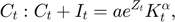
$\mu_{t}: \mu_{t}+\beta\mathrm{E}_{t}\left[a \alpha e^{Z_{t+1}}K_{t+1}^{\alpha-1}C_{t+1}^{-\tau}-\mu_{t+1}\left(1-\delta\right)\right]=0.$

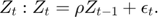
Transition equations

$K_{t}: K_{t}=\left(1-\delta\right)K_{t-1}+I_{t-1},$

$Z_{t}: Z_{t}=\rho Z_{t-1}+\epsilon_{t}.$

Writing the model

The model is defined in a Yaml file: gro2.yaml.

Create the model object

Mean and standard deviation of the shocks

Mu                = 0;
sigma             = 0.04;

model = recsmodel('gro2.yaml',...
                  struct('Mu',Mu,'Sigma',sigma^2,'order',7));

Deterministic steady state (different from first guess, max(|delta|)=4.52137)
 State variables:
    K         Z     
    _    ___________

    1    -3.5818e-19

 Response variables:
       C         I         Mu   
    _______    ______    _______

    0.22117    0.0196    -4.5214

 Expectations variables:
      E   
    ______

    4.7593

This command creates a MATLAB file, gro2model.m, containing the definition the model and all its Jacobians from the human readable file gro2.yaml.

Define approximation space

Degree of approximation

order         = 24;

Limits of the state space

smin          = [0.47*model.sss(1)  min(model.shocks.e)*3.5];
smax          = [1.72*model.sss(1)  max(model.shocks.e)*3.5];

[interp,s] = recsinterpinit(order,smin,smax);

Define options

options = struct('fgmethod','perturbation',...
                 'reesolver','mixed');

Find a first guess through first-order approximation around the steady state

[interp,x] = recsFirstGuess(interp,model,s,model.sss,model.xss,options);

Solve for rational expectations

interp = recsSolveREE(interp,model,s,x,options);

Successive approximation
  Major	 Minor	Lipschitz	 Residual
      0	     0	         	 2.83E+00 (Input point)
      1	     1	  0.5633	 1.55E+00
      2	     1	  0.2903	 1.26E+00
      3	     1	  0.2548	 1.07E+00
      4	     1	  0.2091	 9.38E-01
      5	     1	  0.1813	 8.32E-01
      6	     1	  0.1673	 7.39E-01
      7	     1	  0.1639	 6.52E-01
      8	     1	  0.1603	 5.67E-01
      9	     1	  0.1698	 4.84E-01
     10	     1	  0.1718	 4.08E-01
Too many iterations
Newton-Krylov solver
  Major  Residual  Minor 1  Relative res.  Minor 2
      0  4.08E-01        0       1.00E+00        0 (Input point)
      1  2.00E-01        1       4.91E-01        0
      2  5.21E-02        1       2.60E-01        0
      3  1.61E-02        2       3.09E-01        0
      4  1.97E-03        3       1.22E-01        0
      5  1.74E-05       11       8.87E-03        0
      6  3.94E-09       10       2.26E-04        0

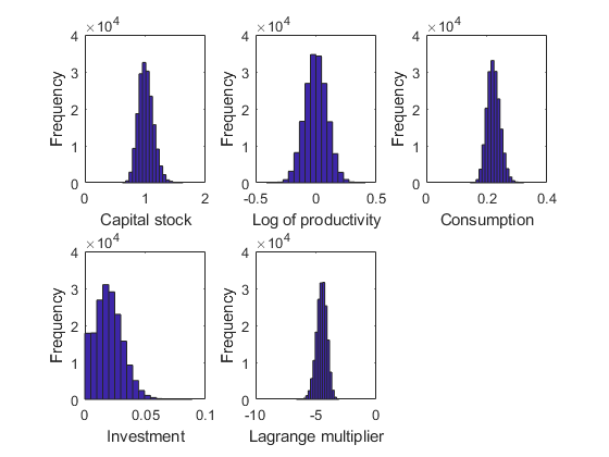
Simulate the model

[~,~,~,stat] = recsSimul(model,interp,model.sss(ones(1000,1),:),200);
subplot(2,3,1)
xlabel('Capital stock')
ylabel('Frequency')
subplot(2,3,2)
xlabel('Log of productivity')
ylabel('Frequency')
subplot(2,3,3)
xlabel('Consumption')
ylabel('Frequency')
subplot(2,3,4)
xlabel('Investment')
ylabel('Frequency')
subplot(2,3,5)
xlabel('Lagrange multiplier')
ylabel('Frequency')

Statistics from simulated variables (excluding the first 20 observations):
 Moments
             Mean         StdDev     Skewness    Kurtosis      Min         Max        pLB      pUB
          ___________    ________    ________    ________    ________    ________    ______    ___

    K          1.0134     0.12252     0.40204     3.247       0.62059      1.6243       NaN    NaN
    Z     -0.00018851    0.091124    0.002673    2.9985      -0.40935     0.41021       NaN    NaN
    C         0.22292    0.021423     0.31764    3.1586       0.14486     0.32353         0      0
    I        0.019893    0.011407     0.44382    3.1573             0    0.089075    1.8717      0
    Mu        -4.5226     0.42991    -0.23494    3.0625       -6.6269     -3.0908         0      0

 Correlation
             K          Z          C          I         Mu   
          _______    _______    _______    _______    _______

    K           1    0.61079    0.95318    0.17578    0.95006
    Z     0.61079          1    0.81869    0.87473    0.80603
    C     0.95318    0.81869          1    0.45494    0.98932
    I     0.17578    0.87473    0.45494          1    0.43491
    Mu    0.95006    0.80603    0.98932    0.43491          1

 Autocorrelation
            T1         T2         T3         T4         T5   
          _______    _______    _______    _______    _______

    K     0.99221    0.97359     0.9463    0.91223    0.87296
    Z     0.87718    0.76803    0.67235    0.58657    0.51116
    C     0.97464    0.94237    0.90489     0.8632    0.81874
    I     0.81983    0.66701    0.53849    0.42835    0.33572
    Mu    0.97783    0.94799    0.91239    0.87211    0.82869

References

Christiano, L.J. and Fisher, J.D.M. (2000). Algorithms for solving dynamic models with occasionally binding constraints. Journal of Economic Dynamics and Control, 24(8), 1179-1232.