STO1 Competitive storage model

This model is a standard competitive storage model with supply reaction. Its setting is close to Wright and Williams (1982).

Model's structure
Writing the model
Create the model object
Define approximation space
Find a first guess through the perfect foresight solution
Solve for rational expectations
Plot the decision rules
Simulate the model
Assess solution accuracy
References

Model's structure

Response variables Storage ( $S$ ), Planned production ( $H$ ) and Price ( $P$ ).

State variable Availability ( $A$ ).

Shock Productivity shocks ( $\epsilon$ ).

Parameters Unit physical storage cost ( $k$ ), Depreciation share ( $\delta$ ), Interest rate ( $r$ ), Scale parameter for the production cost function ( $h$ ), Inverse of supply elasticity ( $\mu$ ) and Demand price elasticity ( $\alpha$ ).

Equilibrium equations

$S_{t}: S_{t}\ge 0 \quad \perp \quad P_{t}+k-\frac{1-\delta}{1+r}\mathrm{E}_{t}\left(P_{t+1}\right)\ge 0,$

$H_{t}: \frac{1}{1+r}\mathrm{E}_{t}\left(P_{t+1}\epsilon_{t+1}\right)=h {H_{t}}^{\mu},$

$P_{t}: A_{t}={P_{t}}^{\alpha}+S_{t}.$

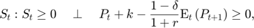
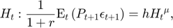
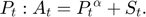
Transition equation

$A_{t}: A_{t}=\left(1-\delta\right)S_{t-1}+H_{t-1}\epsilon_{t}.$

Writing the model

The model is defined in a Yaml file: sto1.yaml.

Create the model object

Mu                = 1;
sigma             = 0.05;

model = recsmodel('sto1.yaml',struct('Mu',Mu,'Sigma',sigma^2,'order',7));

Deterministic steady state (equal to first guess)
 State variables:
    A
    _

    1

 Response variables:
    S    H    P
    _    _    _

    0    1    1

 Expectations variables:
    EP    EPe
    __    ___

    1     1

Define approximation space

[interp,s] = recsinterpinit(40,model.sss*0.7,model.sss*1.5);

Find a first guess through the perfect foresight solution

interp = recsFirstGuess(interp,model,s,model.sss,model.xss,struct('T',5));

Solve for rational expectations

interp = recsSolveREE(interp,model);

Successive approximation
  Major	 Minor	Lipschitz	 Residual
      0	     0	         	 7.18E-02 (Input point)
      1	     1	  0.7774	 4.27E-02
      2	     1	  0.6246	 2.88E-02
      3	     1	  0.5941	 1.22E-02
      4	     1	  0.6840	 3.88E-03
      5	     1	  0.7230	 1.08E-03
      6	     1	  0.7359	 2.84E-04
      7	     1	  0.7394	 7.41E-05
      8	     1	  0.7408	 1.92E-05
      9	     1	  0.7412	 4.97E-06
     10	     1	  0.7412	 1.29E-06
     11	     1	  0.7412	 3.33E-07
     12	     1	  0.7432	 8.58E-08
     13	     1	  0.8677	 1.86E-08
     14	     1	  1.0000	 0.00E+00
Solution found - Residual lower than absolute tolerance

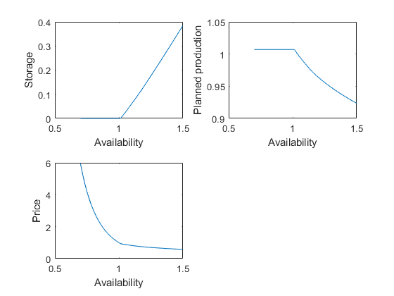
Plot the decision rules

recsDecisionRules(model,interp,[],[],[],struct('simulmethod','solve'));
subplot(2,2,1)
xlabel('Availability')
ylabel('Storage')
subplot(2,2,2)
xlabel('Availability')
ylabel('Planned production')
subplot(2,2,3)
xlabel('Availability')
ylabel('Price')

Simulate the model

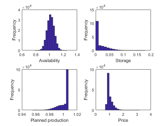
[ssim,~,~,stat] = recsSimul(model,interp,model.sss(ones(1000,1),:),200);
subplot(2,2,1)
xlabel('Availability')
ylabel('Frequency')
subplot(2,2,2)
xlabel('Storage')
ylabel('Frequency')
subplot(2,2,3)
xlabel('Planned production')
ylabel('Frequency')
subplot(2,2,4)
xlabel('Price')
ylabel('Frequency')

Statistics from simulated variables (excluding the first 20 observations):
 Moments
           Mean       StdDev      Skewness    Kurtosis      Min        Max       pLB      pUB
         ________    _________    ________    ________    _______    _______    ______    ___

    A      1.0162     0.051825    0.019719    2.9954      0.79312     1.2528       NaN    NaN
    S    0.015508     0.021954      1.6549    5.5816            0    0.17869    23.972      0
    H       1.001    0.0080711     -1.4145    4.3785       0.9553     1.0072         0      0
    P      1.0164      0.20256      1.8699    7.7434      0.69929     3.1864         0      0

 Correlation
            A           S           H           P   
         ________    ________    ________    _______

    A           1     0.86642    -0.87774    -0.9043
    S     0.86642           1    -0.99794     -0.578
    H    -0.87774    -0.99794           1    0.59579
    P     -0.9043      -0.578     0.59579          1

 Autocorrelation
           T1          T2          T3            T4            T5    
         _______    ________    _________    __________    __________

    A    0.21258    0.041476     0.005918    -0.0079829    -0.0089553
    S    0.24111    0.051096    0.0054768    -0.0092697     -0.010646
    H    0.23996    0.050647    0.0056397    -0.0090575     -0.010316
    P    0.11904    0.016731     0.002795    -0.0061893    -0.0071728

Assess solution accuracy

recsAccuracy(model,interp,ssim);

Accuracy of the solution
 Equilibrium equation error (in log10 units)
    Max       Mean
   -2.2986   -3.1471
   -2.7699   -3.7235
   -3.3881   -4.3433

References

Wright, B. D. and Williams, J. C. (1982). The economic role of commodity storage. The Economic Journal, 92(367), 596-614.

RECS