STO4 Competitive storage with price-band backed by public storage

This model is an extension of Miranda and Helmberger (1988) to include a capacity constraint on the public stock level (see also Gouel 2013).

Model's structure
Writing the model
Create the model object
Multiple steady states
Define approximation space
Find a first guess through the perfect foresight solution
Solve for rational expectations
Simulate the model
References

Model's structure

Response variables Speculative storage ( $S^{\mathrm{S}}$ ), Increase in public stock level ( $\Delta S^{\mathrm{G}+}$ ), Decrease in public stock level ( $\Delta S^{\mathrm{G}-}$ ), Planned production ( $H$ ) and Price ( $P$ ).

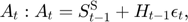
State variable Availability ( $A$ ) and Public stock ( $S^{\mathrm{G}}$ ).

Shock Productivity shocks ( $\epsilon$ ).

Parameters Unit physical storage cost ( $k$ ), Interest rate ( $r$ ), Scale parameter for the production cost function ( $h$ ), Inverse of supply elasticity ( $\mu$ ), Demand price elasticity ( $\alpha$ ), Floor price ( $P^{\mathrm{F}}$ ), Ceiling price ( $P^{\mathrm{c}}$ ) and Capacity constraint on public stock ( $\bar{S}^{\mathrm{G}}$ ).

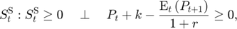
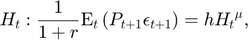
Equilibrium equations

$S^{\mathrm{S}}_{t}: S^{\mathrm{S}}_{t}\ge 0 \quad \perp \quad P_{t}+k-\frac{\mathrm{E}_{t}\left(P_{t+1}\right)}{1+r}\ge 0,$

$H_{t}: \frac{1}{1+r}\mathrm{E}_{t}\left(P_{t+1}\epsilon_{t+1}\right)=h {H_{t}}^{\mu},$

$P_{t}: A_{t}+\Delta S^{\mathrm{G}-}_{t}={P_{t}}^{\alpha}+S^{\mathrm{S}}_{t}+\Delta S^{\mathrm{G}+}_{t},$

$\Delta S^{\mathrm{G}+}_{t}:0\le\Delta S^{\mathrm{G}+}_{t}\le\bar{S}^{\mathrm{G}}-S^{\mathrm{G}}_{t-1} \quad \perp \quad P_{t}-P^{\mathrm{F}},$

$\Delta S^{\mathrm{G}-}_{t}:0\le\Delta S^{\mathrm{G}-}_{t}\le S^{\mathrm{G}}_{t-1} \quad \perp \quad P^{\mathrm{c}}-P_{t}.$

Transition equation

$A_{t}: A_{t}=S^{\mathrm{S}}_{t-1}+H_{t-1}\epsilon_{t},$

$S^{\mathrm{G}}_{t}: S^{\mathrm{G}}_{t}= S^{\mathrm{G}}_{t-1}+\Delta S^{\mathrm{G}+}_{t-1}-\Delta S^{\mathrm{G}-}_{t-1}.$

Writing the model

The model is defined in a Yaml file: sto4.yaml.

Create the model object

Mu                = 1;
sigma             = 0.05;
model = recsmodel('sto4.yaml',struct('Mu',Mu,'Sigma',sigma^2,'order',7));

Deterministic steady state (equal to first guess)
 State variables:
    A    Sg 
    _    ___

    1    0.4

 Response variables:
    S    H    P    DSgp    DSgm
    _    _    _    ____    ____

    0    1    1    0       0   

 Expectations variables:
    EP    EPe
    __    ___

    1     1

Sgbar = model.params(end-1);

Multiple steady states

In this model, there is no stock depreciation. This assumption implies that there are multiple steady states: as long as the steady-state price is between the floor and ceiling prices, any public stock level between 0 and $\bar{S}^{\mathrm{G}}$ is a steady state. Actually, the steady-state response variables are unique, only the public stock level is indeterminate as we can see in the examples below:

[sss1,xss1] = recsSS(model,[1 0],model.xss);

Deterministic steady state (equal to first guess)
 State variables:
    A    Sg
    _    __

    1    0 

 Response variables:
    S    H    P    DSgp    DSgm
    _    _    _    ____    ____

    0    1    1    0       0   

 Expectations variables:
    EP    EPe
    __    ___

    1     1

[sss2,xss2] = recsSS(model,[1 0.2],model.xss);

Deterministic steady state (equal to first guess)
 State variables:
    A    Sg 
    _    ___

    1    0.2

 Response variables:
    S    H    P    DSgp    DSgm
    _    _    _    ____    ____

    0    1    1    0       0   

 Expectations variables:
    EP    EPe
    __    ___

    1     1

Define approximation space

[interp,s] = recsinterpinit(20,[0.74 0],[1.4 Sgbar]);

Find a first guess through the perfect foresight solution

interp = recsFirstGuess(interp,model,s,model.sss,model.xss,struct('T',5));

Solve for rational expectations

[interp,x] = recsSolveREE(interp,model,s);

Successive approximation
  Major	 Minor	Lipschitz	 Residual
      0	     0	         	 1.50E-01 (Input point)
      1	     1	  0.8672	 6.27E-02
      2	     1	  0.6394	 2.84E-02
      3	     1	  0.6901	 8.93E-03
      4	     1	  0.7305	 2.41E-03
      5	     1	  0.7453	 6.14E-04
      6	     1	  0.7509	 1.53E-04
      7	     1	  0.7528	 3.78E-05
      8	     1	  0.7535	 9.32E-06
      9	     1	  0.7537	 2.30E-06
     10	     1	  0.7540	 5.67E-07
     11	     1	  0.7598	 1.40E-07
     12	     1	  0.9398	 3.24E-08
     13	     1	  1.0000	 0.00E+00
Solution found - Residual lower than absolute tolerance

Simulate the model

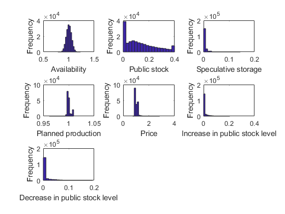
options.stat = 1;
recsSimul(model,interp,repmat([1 0],1E3,1),200,[],options);
subplot(3,3,1)
xlabel('Availability')
ylabel('Frequency')
subplot(3,3,2)
xlabel('Public stock')
ylabel('Frequency')
subplot(3,3,3)
xlabel('Speculative storage')
ylabel('Frequency')
subplot(3,3,4)
xlabel('Planned production')
ylabel('Frequency')
subplot(3,3,5)
xlabel('Price')
ylabel('Frequency')
subplot(3,3,6)
xlabel('Increase in public stock level')
ylabel('Frequency')
subplot(3,3,7)
xlabel('Decrease in public stock level')
ylabel('Frequency')

Statistics from simulated variables (excluding the first 20 observations):
 Moments
              Mean        StdDev      Skewness     Kurtosis      Min        Max       pLB       pUB  
            _________    _________    _________    ________    _______    _______    ______    ______

    A           1.004     0.050486    0.0050016    2.9912      0.78697     1.2316       NaN       NaN
    Sg        0.13528       0.1159      0.67697    2.4411            0        0.4       NaN       NaN
    S       0.0040365    0.0075183       3.7378    27.244            0     0.1444    35.415         0
    H         0.99999    0.0039457      0.54691    6.3107      0.96172     1.0097         0         0
    P           1.007      0.12142       2.1476    13.615      0.74116     2.8374         0         0
    DSgp    0.0092738     0.019729       2.8634    12.165            0    0.20619    38.557    1.0844
    DSgm    0.0089268     0.018965       2.7876    11.426            0    0.19424    26.427    9.2961

 Correlation
                A           Sg           S           H           P          DSgp         DSgm  
            _________    _________    ________    ________    ________    _________    ________

    A               1    -0.052898     0.57932    -0.52389    -0.81646      0.71504    -0.69501
    Sg      -0.052898            1    -0.10746    -0.51905    -0.09671    -0.048125     0.15038
    S         0.57932     -0.10746           1    -0.47524    -0.47195      0.28753    -0.24819
    H        -0.52389     -0.51905    -0.47524           1     0.58195     -0.36285      0.1295
    P        -0.81646     -0.09671    -0.47195     0.58195           1     -0.40827     0.42106
    DSgp      0.71504    -0.048125     0.28753    -0.36285    -0.40827            1    -0.21875
    DSgm     -0.69501      0.15038    -0.24819      0.1295     0.42106     -0.21875           1

 Autocorrelation
               T1           T2            T3           T4            T5    
            ________    __________    __________    _________    __________

    A       0.041787      -0.02014     -0.015863     -0.02007     -0.016676
    Sg       0.93562       0.87078       0.81071      0.75463        0.7032
    S        0.16836      0.067865      0.049235     0.035641      0.030582
    H        0.49457       0.37386       0.31506      0.26788       0.23226
    P       0.079151      0.018209      0.015877      0.01248     0.0091157
    DSgp     0.02324    -0.0068244    -0.0071192    -0.013707     -0.010108
    DSgm    0.015919    -0.0061996    -0.0038683    -0.010361    -0.0059664

References

Gouel, C. (2013). Rules versus discretion in food storage policies. American Journal of Agricultural Economics, 95(4), 1029-1044.

Miranda, M. J. and Helmberger, P. G. (1988). The effects of commodity price stabilization programs. The American Economic Review, 78(1), 46-58.

RECS