Definition of a stochastic rational expectations problem

Rational expectation models

There are several ways to define rational expectations models. RECS adopts a controlled-process convention in which the values taken by control, or response, variables are decided at each period based on the values of state variables. The convention follows the framework proposed in Fackler (2005), and used also in Winschel et Krätzig (2010). A model can be defined by the following three equations, where time subscripts are implicit for current-period variables, and, where next-period are indicated with the $+$ subscript, while previous-period variables are indicated with the $-$ subscript.

$\underline{x}(s) \le x \le \overline{x}(s) \perp f(s,x,z)$, where $f:\mathbf{R}^{d+m+p}\rightarrow \mathbf{R}^{m}$,

$z = \mathrm{E} \left[h(s,x,e_{+},s_{+},x_{+})\right]$, where $h:\mathbf{R}^{d+m+q+d+m}\rightarrow \mathbf{R}^{p}$,

$s = g(s_{-},x_{-},e)$, where $g:\mathbf{R}^{d+m+q}\rightarrow \mathbf{R}^{d}$.

Variables have been partitioned into state variables, $s$, response variables, $x$, and shocks, $e$. Response variables can have lower and upper bounds, $\underline{x}$ and $\overline{x}$, which themselves can be functions of the state variables. Expectations variables, denoted by $z$, are also defined, because they are necessary for solving the model considering the implemented algorithms. $\mathrm{E}$ is the expectations operator conditional on information available at the current period.

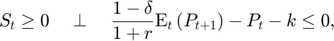
The first equation is the equilibrium equation. It characterizes the behavior of the response variables given state variables and expectations about the next period. For generality, it is expressed as a mixed complementarity problem (MCP, if you aren't familiar with the definition of MCP, see Introduction to mixed complementarity problems). In cases where response variables have no lower and upper bounds, or have infinte ones, it simplifies to a traditional equation:

$0=f(s,x,z)$.

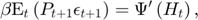
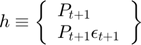
The second equation defines the expectations. The last equation is the state transition equation, which defines how state variables are updated based on past response, past state and contemporaneous shocks.

Restrictions imposed by the RECS convention

Distinction between state variables and other variables

In many models, it is possible to simplify the state transition equation 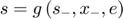$s=g\left(s_{-},x_{-},e\right)$. For example, it is possible to have $s=e$ when some shocks are not serially correlated, or $s=x_{-}$ when the state is just a lagged response variables. In the latter case, one might be tempted to reduce the number of variables in the model by introducing the lagged response variable directly in the equilibrium equation. This should not be done. A state variable corresponding to the lagged response variable or to the realized shock has to be created.

One consequence is that lags can only appear in state transition equations and in no other equations.

Lags and leads

RECS only deals with lags and leads of one period. For a model with lags/leads of more periods, additional variables have to be included to reduce the number of periods.

In addition, leads can only appear in the equations defining expectations. So no leads or lags should ever appear in the equilibrium equations.

Timing convention

In RECS, the timing of each variable reflects when that variable is decided/determined. In particular, the RECS convention implies that state variables are determined by a transition equation that includes shocks and so are always contemporaneous to shocks, even when shocks do not actually play a role in the transition equation. This convention implies that the timing of each variable depends on the way the model is written.

One illustration of the consequences of this convention is the timing of planned production in the competitive storage model presented in STO1. Planned production, $H_{t}$, will only lead to actual production in $t+1$ and will be subject to shocks, $\epsilon_{t+1}$, so it is tempting to use a $t+1$ indexing. However, since it is determined in $t$ based on expectations of period $t+1$ price, it should be indexed $t$.

An example

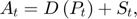
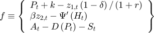
As an example, consider the competitive storage model presented in STO1. It is composed of four equations:

$S_t \ge 0 \quad \perp \quad \frac{1-\delta}{1+r}\mathrm{E}_{t}\left(P_{t+1}\right)-P_{t}-k \le 0,$

$\beta\mathrm{E}_{t}\left(P_{t+1} \epsilon_{t+1}\right)=\Psi'\left(H_{t}\right),$

$A_{t} = D\left(P_{t}\right)+S_t,$

$A_{t}=H_{t-1}\epsilon_{t}+\left(1-\delta\right) S_{t-1},$

where $S$, $H$, $P$, and $A$ respectively represent storage, planned production, price and availability.

There are three response variables: 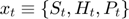$x_{t} \equiv \left\{S_{t},H_{t},P_{t}\right\}$, and three corresponding equilibrium equations, the first three equations above. These equations include two terms corresponding to expectations about period $t+1$: $z_{t} \equiv \left\{\mathrm{E}_{t}\left(P_{t+1}\right),\mathrm{E}_{t}\left(P_{t+1} \epsilon_{t+1}\right)\right\}.$

There is one state variable, availability: $s_{t} \equiv \left\{A_{t}\right\}$, which is associated to the transition equation, the last one above. It would have been perfectly legitimate to define the model with more state variables, such as production and stocks, since availability is the sum of both, and this would not prevent the solver from finding the solution, however, it is generally not a good idea. Since the solution methods implemented in RECS suffer from the curse of dimensionality, it is important where possible to combine predetermined variables to reduce the number of state variables.

Corresponding to RECS convention, this model is defined by the following three functions $\left\{f,h,g\right\}$:

$f \equiv \left\{\begin{array}{l} P_{t}+k-z_{1,t}\left(1-\delta\right)/\left(1+r\right)\\ \beta z_{2,t}-\Psi'\left(H_{t}\right)\\ A_{t}-D\left(P_{t}\right)-S_{t} \end{array} \right\}$

$h \equiv \left\{\begin{array}{l} P_{t+1}\\ P_{t+1}\epsilon_{t+1} \end{array} \right\}$

$g \equiv \left\{ H_{t-1}\epsilon_{t}+\left(1-\delta\right)S_{t-1}\right\}$

Solving a rational expectations model

What makes solving a rational expectations model complicated is that the equation defining the expectations, $z = \mathrm{E}_{e_{+}} \left[h(s,x,e_{+},s_{+},x_{+})\right]$, is not a traditional algebraic equation. It is an equation that expresses the consistency between agents' expectations, their information set, and realized outcomes.

One way to bring this problem back to a traditional equation is to find an approximation or an algebraic representation of the expectations terms. For example, if it is possible to find an approximation of the relationship between expectations and current-period state variables (i.e., the parameterized expectations approach in den Haan and Marcet, 1990), the equilibrium equation can be simplified to

$\underline{x}(s) \le x \le \overline{x}(s) \perp f\left(s,x,\mathcal{Z}\left(s,c_z\right)\right),$

where $\mathcal{Z}\left(s,c_{z}\right)$ approximates the expectations $z$ and $c_{z}$ are the coefficients characterizing this approximation. This equation can be solved for $x$ with any MCP solvers.

The RECS solver implements various methods to solve rational expectations models and to find approximation for the expectations terms. See Solution methods for further information.

References

Fackler, P. L. (2005). A MATLAB Solver for Nonlinear Rational Expectations Models. Computational Economics, 26(2), 173-181.

Winschel, V. and Krätzig, M. (2010). Solving, Estimating, and Selecting Nonlinear Dynamic Models Without the Curse of Dimensionality. Econometrica, 78(2), 803-821.

den Haan, W. J. and Marcet, A. (1990). Solving the Stochastic Growth Model by Parameterizing Expectations. Journal of Business & Economic Statistics, 8(1), 31-34.