STO6SP Quarterly storage model with informational subperiods and annual inelastic supply
This model represents the market of a storable commodity that is produced once a year and stored for a year-long consumption. Supply is stochastic and inelastic. Contrary to STO6, there are informational shocks about the coming harvest that allows stocks to be adjusted before the full harvest is known.
Contents
Writing the model
The model is defined in 4 Yaml files: sto6SP1.yaml, sto6SP2.yaml, sto6SP3.yaml, and sto6SP4.yaml.
Create the model object
model = recsmodelsp({'sto6SP1.yaml' 'sto6SP2.yaml' 'sto6SP3.yaml' 'sto6SP4.yaml'});
model.shocks = cell(model.nperiods,1);
model.bounds = cell(model.nperiods,2);

params = num2cell(model.params);
[k, delta, r, elastD, d] = params{:};
Define approximation space and shocks
clear('interp')
sigma = [0.05 eps eps eps];
n     = {50; 50; [50 5]; [50 5]};
smin  = {2.8; 2.05; [1.35 -0.15]; [0.67 -0.21]};
smax  = {6  ; 5.1 ; [3.9   0.15]; [2.72  0.21]};
for iperiod=1:model.nperiods
  % Shocks
  [model.shocks{iperiod}.e,model.shocks{iperiod}.w] = qnwnorm(5,0,sigma(iperiod)^2);
  model.shocks{iperiod}.funrand = @(nrep) randn(nrep,1)*sigma(iperiod);
end
% Interpolation structure
interp.fspace = cellfun(@(N,SMIN,SMAX) fundefn('spli',N,SMIN,SMAX),n,smin,smax,...
                        'UniformOutput', false);
interp.Phi    = cellfun(@(FSPACE) funbasx(FSPACE),interp.fspace,...
                        'UniformOutput', false);
interp.s      = cellfun(@(FSPACE) gridmake(funnode(FSPACE)),interp.fspace,...
                        'UniformOutput', false);

[model.ss.sss,model.ss.xss,model.ss.zss] = recsSSSP(model,{4; 3; [2 0]; [1 0]},...
                                                  {[3 1]; [2 1]; [1 1]; [0 1]});

[s1,s2,s3,s4] = interp.s{:};
Deterministic steady state (different from first guess, max(|delta|)=0.0961408)
 State variables:
    A1      A2        A3        E3Prod        A4         E4Prod
    __    ______    ______    __________    _______    __________

    4     2.9815    1.9756    1.4452e-19    0.98181    2.8904e-19

 Response variables:
      S1        P1         S2        P2        S3         P3          S4          P4
    ______    _______    ______    ______    _______    ______    __________    ______

    2.9964    0.98214    1.9854    1.0197    0.98671    1.0577    1.3361e-18    1.0961

 Expectations variables:
		1.02	1.058	1.096	0.9821
Bounds
for iperiod=1:model.nperiods
  [LB,UB] = eval(['model.functions(iperiod).b(s' int2str(iperiod) '(1,:),params);']);
  model.bounds(iperiod,:) = {LB UB};
end
Provide a simple first guess
x4 = [zeros(size(s4,1),1)     (s4(:,1)/d).^(1/elastD)];
x3 = [s3(:,1)/2           ((s3(:,1)/2)/d).^(1/elastD)];
x2 = [s2(:,1)*2/3         ((s2(:,1)/3)/d).^(1/elastD)];
x1 = [s1(:,1)*3/4         ((s1(:,1)/4)/d).^(1/elastD)];
Solve for rational expectations
[interp,X] = recsSolveREESP(model,interp,{x1; x2; x3; x4});
Successive approximation
   Iter	Residual
      1	1.65E+01
      2	2.49E+00
      3	9.37E-01
      4	3.33E-01
      5	1.06E-01
      6	2.99E-02
      7	8.06E-03
      8	2.21E-03
      9	6.19E-04
     10	1.75E-04
     11	4.95E-05
     12	1.41E-05
     13	3.99E-06
     14	1.13E-06
     15	0.00E+00
Solution found - Residual lower than absolute tolerance
Compare STO6 and STO6SP when informational shocks are removed
if exist('Xcat','var')
  disp('Max absolute error in first subperiod storage and price (in log10)');
  disp(log10(max(abs(Xcat(:,[1 5])-X{1}))));
end
Introduced information shocks
sigma = [0.05/sqrt(3) eps 0.05/sqrt(3) 0.05/sqrt(3)];
for iperiod=1:model.nperiods
  % Shocks
  [model.shocks{iperiod}.e,model.shocks{iperiod}.w] = qnwnorm(5,0,sigma(iperiod)^2);
  model.shocks{iperiod}.funrand = @(nrep) randn(nrep,1)*sigma(iperiod);
end

[interp,X] = recsSolveREESP(model,interp,X);

[ssim,xsim,esim,stat,fsim] = recsSimulSP(model,interp,repmat(4,1000,1),200);
Successive approximation
Iter Residual
1 4.74E-01
2 8.75E-02
3 3.68E-02
4 1.66E-02
5 6.33E-03
6 2.93E-03
7 1.30E-03
8 3.96E-04
9 9.84E-05
10 2.22E-05
11 4.79E-06
12 1.00E-06
13 0.00E+00
Solution found - Residual lower than absolute tolerance
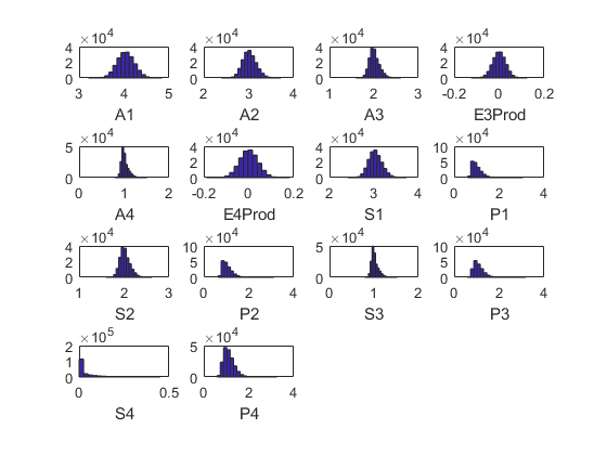
Statistics from simulated variables (excluding the first 20 observations):
Moments
Mean StdDev Skewness Kurtosis Min Max pLB pUB
__________ ________ __________ ________ ________ _______ ______ ___
A1 4.0357 0.19163 0.06465 2.9878 3.2041 4.8393 NaN NaN
A2 3.0171 0.15235 0.24829 3.1312 2.3922 3.713 NaN NaN
A3 2.011 0.11496 0.5569 3.5013 1.5876 2.604 NaN NaN
E3Prod 5.4327e-05 0.028824 -0.010354 3.0155 -0.12376 0.1235 NaN NaN
A4 1.017 0.080443 1.1514 4.662 0.79025 1.5146 NaN NaN
E4Prod 7.3159e-05 0.040745 -0.0014506 2.9953 -0.18843 0.18086 NaN NaN
S1 3.0321 0.15311 0.24829 3.1312 2.4041 3.7315 0 0
P1 1.0066 0.21537 1.2864 5.3842 0.59948 3.0522 0 0
S2 2.0211 0.11554 0.5569 3.5013 1.5955 2.617 0 0
P2 1.0444 0.21805 1.2863 5.384 0.63226 3.1154 0 0
S3 1.022 0.080844 1.1514 4.662 0.79419 1.5221 0 0
P3 1.0825 0.22712 1.114 4.9948 0.58569 3.1812 0 0
S4 0.035603 0.054246 2.1135 7.9023 0 0.45079 30.347 0
P4 1.1208 0.24161 0.95138 4.4806 0.58498 3.2488 0 0
Correlation
A1 A2 A3 E3Prod A4 E4Prod S1 P1 S2 P2 S3 P3 S4 P4
_________ _________ _________ __________ _________ __________ _________ __________ _________ __________ _________ ________ ________ ________
A1 1 0.99899 0.993 0.0024029 0.95869 0.0019429 0.99899 -0.95003 0.993 -0.95002 0.95869 -0.92397 0.75093 -0.87923
A2 0.99899 1 0.99731 0.0023972 0.969 0.0018378 1 -0.9359 0.99731 -0.93589 0.969 -0.91024 0.77226 -0.8661
A3 0.993 0.99731 1 0.0023819 0.98161 0.0016637 0.99731 -0.90876 1 -0.90874 0.98161 -0.88385 0.80368 -0.84089
E3Prod 0.0024029 0.0023972 0.0023819 1 -0.11245 0.70601 0.0023972 -0.0019278 0.0023819 -0.0019207 -0.11245 -0.20571 -0.29709 -0.18088
A4 0.95869 0.969 0.98161 -0.11245 1 -0.079773 0.969 -0.83724 0.98161 -0.83721 1 -0.78345 0.8922 -0.74626
E4Prod 0.0019429 0.0018378 0.0016637 0.70601 -0.079773 1 0.0018378 -0.0020694 0.0016637 -0.0020625 -0.079773 -0.14606 -0.34886 -0.31266
S1 0.99899 1 0.99731 0.0023972 0.969 0.0018378 1 -0.9359 0.99731 -0.93589 0.969 -0.91024 0.77226 -0.8661
P1 -0.95003 -0.9359 -0.90876 -0.0019278 -0.83724 -0.0020694 -0.9359 1 -0.90876 1 -0.83724 0.9725 -0.57003 0.92613
S2 0.993 0.99731 1 0.0023819 0.98161 0.0016637 0.99731 -0.90876 1 -0.90874 0.98161 -0.88385 0.80368 -0.84089
P2 -0.95002 -0.93589 -0.90874 -0.0019207 -0.83721 -0.0020625 -0.93589 1 -0.90874 1 -0.83721 0.9725 -0.56999 0.92613
S3 0.95869 0.969 0.98161 -0.11245 1 -0.079773 0.969 -0.83724 0.98161 -0.83721 1 -0.78345 0.8922 -0.74626
P3 -0.92397 -0.91024 -0.88385 -0.20571 -0.78345 -0.14606 -0.91024 0.9725 -0.88385 0.9725 -0.78345 1 -0.4711 0.94984
S4 0.75093 0.77226 0.80368 -0.29709 0.8922 -0.34886 0.77226 -0.57003 0.80368 -0.56999 0.8922 -0.4711 1 -0.37586
P4 -0.87923 -0.8661 -0.84089 -0.18088 -0.74626 -0.31266 -0.8661 0.92613 -0.84089 0.92613 -0.74626 0.94984 -0.37586 1
Autocorrelation
T1 T2 T3 T4 T5
__________ __________ ___________ __________ __________
A1 0.20153 0.032782 0.00042194 -0.011956 -0.0074951
A2 0.20676 0.034361 0.00044046 -0.012175 -0.0076794
A3 0.21394 0.03655 0.00037985 -0.012522 -0.0079722
E3Prod -0.0040931 -0.0078807 -0.0050107 -0.0063428 -0.0047748
A4 0.16634 0.028203 -0.0014939 -0.012323 -0.0076489
E4Prod -0.0036683 -0.0073908 -0.0055611 -0.0073471 -0.0060193
S1 0.20676 0.034361 0.00044046 -0.012175 -0.0076794
P1 0.15238 0.018343 -0.00087912 -0.010131 -0.0064648
S2 0.21394 0.03655 0.00037985 -0.012522 -0.0079722
P2 0.15236 0.01833 -0.00088855 -0.010136 -0.0064651
S3 0.16634 0.028203 -0.0014939 -0.012323 -0.0076489
P3 0.23653 0.035239 0.0010105 -0.010435 -0.0081844
S4 0.00693 -0.0015752 -0.0066936 -0.010341 -0.0091342
P4 0.34143 0.046942 0.0011096 -0.0097003 -0.0088653