Introduction to mixed complementarity problems
To be able to reliably solve models with occasionally binding constraints, all equilibrium equations should be represented in RECS as mixed complementarity problems (MCP). Here, we present a short introduction to this kind of problems. For more information, see Rutherford (1995), and Ferris and Pang (1997).
Contents
Definition of a mixed complementarity problem
Complementarity problems can be seen as extensions of square systems of nonlinear equations that incorporate a mixture of equations and inequalities. Many economic problems can be expressed as complementarity problems. An MCP is defined as follows (adapted from Munson, 2002):
Definition (Mixed Complementarity Problem) Given a continuously differentiable function  , and lower and upper bounds
The mixed complementarity problem  is to find a
  such that one of the following holds for each
 and
and  ,
,
 and
and  ,
,
 and
and  .
.
To summarize, an MCP problem associates each variable,  , to a lower bound,
  , an upper bound,
  , and an equation,
  . The solution is such that if is between its bounds then . If is equal to its lower (upper) bound then is positive (negative).
This format encompasses several cases. In particular, it is easy to see that with infinite lower and upper bounds, solving an MCP problem is equivalent to solving a square system of nonlinear equations:

A simple example of mixed complementarity
We consider here the traditional consumption/saving problem with borrowing constraint (Deaton, 1991). This problem is solved as a demonstration, see CS1. A consumer with utility  has a stochastic income,
  and has to choose each period how much to consume and how much to save. He is prevented from borrowing, but can save at the rate
  . Without the borrowing constraint, his problem consists of choosing its consumption
  such that it satisfies the standard Euler equation:
![$$u'\left(C_{t}\right)=\frac{1+r}{1+\delta}\mathrm{E}_{t}\left[u'\left(C_{t+1}\right)\right].$$](MCP_eq15521813229849507959.png)
The borrowing constraint implies the inequality  , where
  is the cash on hand available in period
  and defined as

When the constraint is binding (i.e.,  ), the Euler equation no longer holds. The consumer would like to borrow but cannot, so its marginal utility of immediate consumption is higher than its discounted marginal utility over future consumption:
![$$u'\left(C_{t}\right) \ge \frac{1+r}{1+\delta}\mathrm{E}_{t}\left[u'\left(C_{t+1}\right)\right].$$](MCP_eq14883060391907163537.png)
Since the Euler equation holds when consumption is not constrained, this behavior can be summarized by the following complementarity equation
![$$C_{t}\le X_{t} \quad \perp \quad \frac{1+r}{1+\delta}\mathrm{E}_{t}\left[u'\left(C_{t+1}\right)\right]\le u'\left(C_{t}\right).$$](MCP_eq04873718253661185335.png)
When do complementarity problems arise?
In addition to encompassing nonlinear systems of equations, complementarity problems appear naturally in economics. Although not exhaustive, we provide here a few situations that lead to complementarity problems:
- Karush-Kuhn-Tucker conditions of a constrained nonlinear program. The first-order conditions of the following nonlinear programming problem
 subject to
  and
and  can be written as a system of complementarity equations:
  and
and  , where
  is the Lagrange multiplier on the first inequality constraint.
 - Natural representation of regime-switching behaviors. Let us consider two examples. First, a variable
 that is determined as a function of another variable
  as long as is superior to a lower bound
  . Put simply:
 ![$y=\max\left[a,\lambda\left(x\right)\right]$](MCP_eq00421618987462198950.png) . In MCP, we would write this as
. In MCP, we would write this as  . Second, a system of intervention prices in which a public stock is accumulated when prices decrease below the intervention price and sold when they exceed the intervention price (see also STO2) can be represented as
  , where
  ,
,  and
and  , respectively, are the public storage, the price and the intervention price.
 - A Walrasian equilibrium can be formulated as a complementarity problem (Mathiesen, 1987) by associating three sets of variables to three sets of inequalities: non-negative levels of activity are associated to zero-profit conditions, non-negative prices are associated to market clearance, and income levels are associated to income balance.
Conventions of notations adopted for representing and solving complementarity problems
To solve complementarity problems, RECS uses several solvers listed in MCP solvers. The convention adopted in most MCP solvers and used by RECS is the one used above in the MCP definition: superior or equal inequalities are associated with the lower bounds and inferior or equal inequalities are associated with the upper bounds. So, when defining your model, take care to respect this convention.
In addition, in Yaml files inequalities should not be written explicitly. As an example, let's consider these 5 equations:

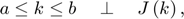
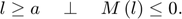
They would be written in a Yaml file as
  - F(x)=0 | -inf<=x<=inf
  - G(y)   |    a<=y<=inf
  - H(z)   | -inf<=z<=b
  - J(k)   |    a<=k<=b
  - -M(l)  |    a<=l<=inf
Note that it is necessary to associate lower and upper bounds with every variables, and the "perp" symbol ( ) is substituted by the vertical bar (|). So if there are no finite bounds, one has to associate infinite bounds. The last equation does not respect the convention that associates lower bounds on variables with superior or equal inequality, so, when writing it in the Yaml file, the sign of the equation needs to be reversed.
References
Deaton, A. (1991). Saving and liquidity constraints. Econometrica, 59(5), 1221-1248.
Munson, T. (2002). Algorithms and Environments for Complementarity. Unpublished PhD thesis from University of Wisconsin, Madison.