Simulate the model

Running a simulation
Choice of simulation techniques
References

Running a simulation

Once the rational expectations equilibrium has been found, it is possible to simulate the model using the function recsSimul with the following call:

[ssim,xsim] = recsSimul(model,interp,s0,nper);

where model and interp have been defined previously as the model object and the interpolation structure. s0 is the initial state and nper is the number of simulation periods.

s0 is not necessarily a unique vector of the state variables. It is possible to provide a matrix of initial states on the basis of which simulations can be run for nper periods. Even starting from a unique state, using this feature will speed up the simulations.

Shocks

The shocks used in the simulation can be provided as the fifth input to the function:

[ssim,xsim] = recsSimul(model,interp,s0,nper,shocks);

However, by default, recsSimul uses the function funrand defined in the model object (see Define the model object) to draw random shocks. If this function is not provided random draws are made from the shock discretization, using the associated probabilities.

To reproduce previously run results, it is necessarily to reset the random number generator using the MATLAB function rng.

Asymptotic statistics

If in the options the field stat is set to 1, or if four arguments are required as the output of recsSimul, then some statistics over the asymptotic distribution are calculated. The first 20 observations are discarded (the number of burn-in observations can be adjusted in the options). The statistics calculated are the mean, standard deviation, skewness, kurtosis, minimum, maximum, percentage of time spent at the lower and upper bounds, correlation matrix, and the five first-order autocorrelation coefficients. In addition, recsSimul draws the histograms of the variables distribution.

These statistics are available as a structure in the fourth output of recsSimul:

[ssim,xsim,esim,stat] = recsSimul(model,interp,s0,nper);

Choice of simulation techniques

There are two main approaches to simulate the model once an approximated rational expectations equilibrium has been found.

Using approximated decision rule

The first, and most common, method consists of simulating the model by applying the approximated decision rules recursively.

Starting from a known $s_1$ , for $t=1:T$

$x_t=\mathcal{X}\left(s_t,c_{x}\right)$

Draw a shock realization $e_{t+1}$ from its distribution and update the state variable:

$s_{t+1}=g\left(s_t,x_t,e_{t+1}\right)$

This is the default simulation method. It is chosen in the options structure by setting the field simulmethod to interpolation.

Solve equilibrium equations using approximated expectations

The second method uses the function being approximated (decisions rules, conditional expectations, or expectations function as shown in Solution methods) to approximate next-period expectations and solve the equilibrium equations to find the current decisions (in a time-iteration approach). For example, if approximated expectations ( $z\approx\mathcal{Z}\left(s,c_z\right)$ ) are used to replace conditional expectations in the equilibrium equation, the algorithm runs as follows:

Starting from a known $s_1$ , for $t=1:T$ , find $x_t$ by solving the following MCP equation using as first guess $x_t=\mathcal{X}\left(s_t,c_{x}\right)$

$\underline{x}(s_t) \le x_t \le \overline{x}(s_t) \perp f\left(s_t,x_t,\mathcal{Z}\left(s_t,c_z\right)\right)$

Draw a shock realization $e_{t+1}$ from its distribution and update the state variable:

$s_{t+1}=g\left(s_t,x_t,e_{t+1}\right)$

This simulation method is chosen in the options structure by setting the field simulmethod to solve.

The two approaches differ in their speed and in precision. Simulating a model through the recursive application of approximated decision rules is very fast because it does not require solving nonlinear equations. The second approach is slower because each period requires that a system of complementarity equations be solved. However, its level of precision is much higher, because the approximation is used only for the expectations of next-period conditions. The precision gain is even more important when decision rules have kinks, which makes them difficult to approximate. Wright and Williams (1984), who first proposed the parameterized expectations algorithm, suggest using the second method to simulate the storage model.

When does this distinction matter?

Most of the time, the default approach of recursively applying the approximated decision rules should be used. Simulating the model by solving the equations should be considered in the following two cases:

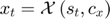
If the model has been solved with low precision, using the approximated decision rules can lead to large errors, while simulating the model by solving the equilibrium equations using only the approximation in expectations will yield a more precise solution. This applies to the following example inspired from STO2: a price-floor policy backed by public storage. If the problem is approximated by a spline with a small grid of 6 points, it is not possible to expect a good approximation of the highly nonlinear storage rules. However, if the approximation is used only in expectations, it yields a very precise solution:

If you are interested in the percentage of time spent in various regimes, solving the equilibrium equations is the only way to achieve a precise estimate. Even when solved with high precision, a simulation using the approximated decision rules provides limited precision regarding the percentage of time spent in each regime. Indeed, approximations using spline or Chebyshev polynomials fluctuate around the exact value between collocation nodes. So between two nodes at which the model should be at a bound, the approximated decision rule can yield a result very close to the bound without actually satisfying it. Below are the moments obtained from simulating the model in STO2 with both methods and with decision rules approximated on 30 nodes. The moments are quite similar, but the approximated decision rules widely underestimate the time spent at the bounds:

Long-run statistics from equilibrium equations solve
Statistics from simulated variables (excluding the first 20 observations):
 Moments
             Mean        StdDev      Skewness    Kurtosis      Min        Max       pLB      pUB 
          __________    _________    ________    ________    _______    _______    ______    ____

    A         1.2354      0.11978    -0.24639    2.3466      0.84566     1.5736       NaN     NaN
    S     0.00067907    0.0049791      9.6845    115.15            0    0.11333    96.467       0
    H         1.0026    0.0048614    -0.79925    6.7045      0.96668      1.016         0       0
    P         1.0149     0.052212      3.5276    65.956      0.74627     2.3121         0       0
    Sg       0.23738      0.11396    -0.33273    2.0936            0        0.4     2.327    8.04

 Correlation
             A           S           H           P           Sg   
          ________    ________    ________    ________    ________

    A            1     0.27432    -0.83925    -0.49432     0.99472
    S      0.27432           1     -0.4932    -0.49417     0.19462
    H     -0.83925     -0.4932           1     0.66962    -0.79911
    P     -0.49432    -0.49417     0.66962           1    -0.41307
    Sg     0.99472     0.19462    -0.79911    -0.41307           1

 Autocorrelation
            T1         T2         T3          T4          T5   
          _______    _______    _______    ________    ________

    A     0.86094    0.74627    0.64798     0.56185     0.48685
    S     0.21177    0.13844    0.12202     0.11063     0.10321
    H     0.67064    0.49358     0.3821     0.30733     0.25496
    P     0.27252    0.15933     0.1057    0.077667    0.057918
    Sg     0.8704    0.75827    0.66079     0.57406     0.49735

Long-run statistics if simulated with approximated decision rules
Statistics from simulated variables (excluding the first 20 observations):
 Moments
             Mean        StdDev      Skewness    Kurtosis      Min        Max       pLB       pUB 
          __________    _________    ________    ________    _______    _______    ______    _____

    A         1.2351      0.11989    -0.24965    2.3483      0.84579     1.5726       NaN      NaN
    S     0.00081005     0.004967       9.378     111.6            0    0.11245    48.809        0
    H         1.0026    0.0049023    -0.73036    6.6906      0.96688     1.0163         0        0
    P         1.0144     0.051055      4.2926    74.372       0.7466     2.3105         0        0
    Sg       0.23685      0.11395    -0.34311    2.0993            0        0.4       1.6    4.554

 Correlation
             A           S           H           P           Sg   
          ________    ________    ________    ________    ________

    A            1     0.31155    -0.84109    -0.49756     0.99474
    S      0.31155           1    -0.53531    -0.54196        0.23
    H     -0.84109    -0.53531           1     0.68384    -0.79965
    P     -0.49756    -0.54196     0.68384           1    -0.41687
    Sg     0.99474        0.23    -0.79965    -0.41687           1

 Autocorrelation
            T1          T2          T3          T4          T5   
          _______    ________    ________    ________    ________

    A     0.86117     0.74661     0.64837     0.56223     0.48724
    S     0.18215    0.083958    0.049018     0.03095    0.020311
    H     0.67101     0.49373     0.38144     0.30733     0.25531
    P     0.29154        0.16     0.10056    0.069375    0.051621
    Sg    0.87074     0.75876     0.66132     0.57462     0.49791

References

Wright, B. D. and Williams, J. C. (1984). The Welfare Effects of the Introduction of Storage. The Quarterly Journal of Economics, 99(1), 169-192.

RECS

Simulate the model

Contents

Running a simulation

Choice of simulation techniques

References