STO3 Anticipated switch to a public storage policy

We consider here the transitional dynamics that occurs when a public storage policy defending a floor price is announced a few periods before its beginning. This is a finite-horizon problem in which the terminal condition is not a unique situation, but a state-contingent policy function. This is a transition from problem STO1 to STO2.

Create the model objects
Define approximation space
Terminal condition: solve for the infinite-horizon behavior under policy
Transition: model without policy in finite horizon
Initial period: model without policy under infinite horizon
Plot price function

Create the model objects

Mu                = 1;
sigma             = 0.05;

Competitive storage model:

model1 = recsmodel('sto1.yaml',struct('Mu',Mu,'Sigma',sigma^2,'order',7));

Deterministic steady state (equal to first guess)
 State variables:
    A
    _

    1

 Response variables:
    S    H    P
    _    _    _

    0    1    1

 Expectations variables:
    EP    EPe
    __    ___

    1     1

Floor price model:

model2 = recsmodel('sto2.yaml',struct('Mu',Mu,'Sigma',sigma^2,'order',7));

Deterministic steady state (different from first guess, max(|delta|)=0.392101)
 State variables:
      A   
    ______

    1.3921

 Response variables:
        S           H       P        Sg   
    __________    _____    ____    _______

    6.0863e-15    1.004    1.02    0.39605

 Expectations variables:
     EP     EPe 
    ____    ____

    1.02    1.02

Define approximation space

[interp,s] = recsinterpinit(50,min(model1.shocks.e)*0.95,2);

Terminal condition: solve for the infinite-horizon behavior under policy

See STO2 for details.

Find a first guess through the perfect foresight solution

interp2 = recsFirstGuess(interp,model2,s,[],[],struct('T',5));

Solve for rational expectations

[~,x2] = recsSolveREE(interp2,model2,s);

Successive approximation
  Major	 Minor	Lipschitz	 Residual
      0	     0	         	 3.69E-02 (Input point)
      1	     1	  1.0414	 1.57E-02
      2	     1	  0.9613	 9.43E-03
      3	     1	  1.0446	 1.89E-03
      4	     1	  0.9479	 1.06E-03
      5	     1	  0.7874	 2.30E-04
      6	     1	  0.8447	 3.57E-05
      7	     1	  0.8511	 5.32E-06
      8	     1	  0.8498	 7.99E-07
      9	     1	  0.8489	 1.21E-07
     10	     1	  0.8483	 1.84E-08
     11	     1	  1.0000	 0.00E+00
Solution found - Residual lower than absolute tolerance

Transition: model without policy in finite horizon

The policy is announced 6 periods before it begins (so $T=7$ ). In the seventh period, the equilibrium is the one defined by the problem with public storage:

T          = 7;
xT         = x2(:,1:3);
options.eqsolver = 'ncpsolve'; % lmmcp does not work in this case
[~,X]  = recsSolveREEFiniteHorizon(interp,model1,s,x2(:,1:3),xT,T,options);

Initial period: model without policy under infinite horizon

In period 0, the policy is not expected by the agents and the prevailing equilibrium is the one corresponding to the infinite-horizon competitive storage problem (STO1):

[~,x1] = recsSolveREE(interp,model1,s,X(:,1:3,1));

Successive approximation
  Major	 Minor	Lipschitz	 Residual
      0	     0	         	 3.64E-02 (Input point)
      1	     1	  0.8292	 6.25E-03
      2	     1	  0.7825	 1.36E-03
      3	     1	  0.7646	 3.20E-04
      4	     1	  0.7589	 7.72E-05
      5	     1	  0.7572	 1.87E-05
      6	     1	  0.7567	 4.56E-06
      7	     1	  0.7565	 1.11E-06
      8	     1	  0.7565	 2.70E-07
      9	     1	  0.7565	 6.58E-08
     10	     1	  0.7565	 1.60E-08
     11	     1	  1.0000	 0.00E+00
Solution found - Residual lower than absolute tolerance

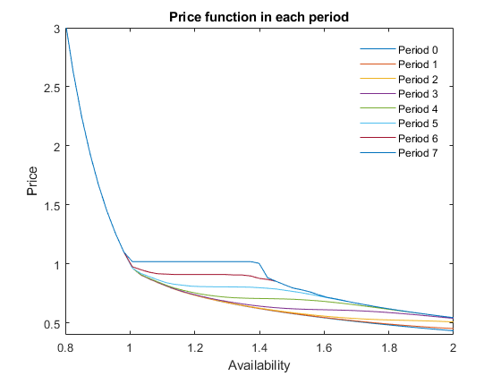
Plot price function

figure
plot(s,[x1(:,3) squeeze(X(:,3,:))])
xlim([0.8 2])
ylim([0.4 3])
legend([repmat('Period ',T+1,1),num2str((0:T)')])
legend('Location','NorthEast')
legend('boxoff')
xlabel('Availability')
ylabel('Price')
title('Price function in each period')

RECS