Writing RECS model files
Structure of a rational expectation models
Before starting to write the model file, you need to organize your equations as described in Definition of a stochastic rational expectations problem. This means that you need to identify and separate in your model the following three group of equations:
Equilibrium equations

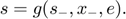
Expectations definition
![$$z = \mathrm{E} \left[h(s,x,e_{+},s_{+},x_{+})\right].$$](ug_model_files_eq15879041859200574127.png)
Transition equations
When defining your model, it is important to try to minimize the number of state variables. Currently, RECS relies for interpolation on grids constructed with tensor products, so the dimension of the problem increases exponentially with the number of state variables. This implies that RECS should be used only to solve small-scale models: more than three or four state variables may make the problems too large to handle. One way of reducing the problem size is, whenever possible, to sum together the predetermined variables that can be summed. You can see in the demonstrations files (e.g., CS1 or STO1) that states variables are occasionaly defined as sums of other predetermined variables.
Structure of RECS model files
An RECS model can be written in a way that is quite similar to the original mathematical notations (as is proposed in most algebraic modeling languages). The model file that must be created is called a Yaml file (because it is written in YAML and has the .yaml extension). A Yaml file is easily readable by human, but not by MATLAB. So the file needs to be processed for MATLAB to be able to read it. This is done by the function recsmodel, which uses a Python preprocessor, dolo-recs, to do the job.
RECS Yaml files require three basic components, written successively:
- declarations - The block declarations contains the declaration of all the variables, shocks and parameters that are used in the model. Inside this block, there are five sub-blocks: states, controls, expectations, shocks, and parameters with corresponding elements declarations.
- equations - The block equations declares model's equations.
- calibration - The block calibration provides numerical values for parameters and a first-guess for the deterministic steady-state.
Yaml file structure
To illustrate a complete Yaml file let us consider how to write a standard stochastic growth model in Yaml (see GRO1 for the complete example):
declarations:
states: [K, Z]
controls: [C]
expectations: [E]
shocks: [Epsilon]
parameters: [a, tau, delta, beta, rho, alpha]
equations:
arbitrage:
- C^(-tau)-beta*E=0 | -inf <= C <= inf
transition:
    - K = a*exp(Z(-1))*K(-1)^alpha+(1-delta)*K(-1)-C(-1)
    - Z = rho*Z(-1)+Epsilon
expectation:
- E = C(1)^(-tau)*(1-delta+a*alpha*exp(Z(1))*K(1)^(alpha-1))
calibration:
parameters:
    tau   : 2
    delta : 0.0196
    beta  : 0.95
    rho   : 0.9
    alpha : 0.33
    a     : (1/beta-1+delta)/alpha
steady_state:
    Z : 0
    K : 1
    C : a-delta
    E : C^(-tau)/beta
See Demos for other examples of complete yaml files.
Yaml files can be written with any text editor, including MATLAB editor.
Yaml syntax conventions
For the file to be readable, it is necessary to respect some syntax conventions:
- Association equilibrium equations/control variables/bounds: Each equilibrium equation must be associated with a control variable. This matters absolutely for equations with complementarity constraints. For traditional equations, the precise association does not matter. The equation and its associated variable are separated by the symbol |. Control variables must be associated with bounds, which can be infinite.
- Indentation: Inside each block, elements of the same scope have to be indented using the same number of spaces (do not use tabs). For the above example, inside the declarations block, states, controls, expectations, shocks, and parameters are indented to the same level.
- Each equation starts with a dash and a space ("- "), not to be confused with a minus sign. To avoid confusion, it is possible instead to use two points and a space (".. "), or two dashes and a space ("-- ").
- Comments: Comments are introduced by the character #.
- Lead/Lag: Lead variables are indicated X(1) and lag variables X(-1).
- Timing convention: Transition equations are written by defining the new state variable at current time as a function of lagged response and state variables:
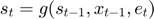 .
. - Do not use lambda as a variable/parameter name, this is a restricted word.
- Write equations in the same order as the order of variables declaration.
- Yaml files are case sensitive.